- P-ISSN 2586-2995
- E-ISSN 2586-4130

To investigate the causes of Korea’s growth slowdown over the past thirty years, we estimate the contributions of major developmental factors, including i) demographic factors (changes in population growth and workforce age due to the demographic transition), ii) quality-of-life-related choice factors (changes in working hours, education, and the female employment rate), iii) structural change, and iv) the effects of productivity catch-up. Our estimates show that these four groups of factors account for approximately 90 percent of the growth slowdown, with demographic factors contributing approximately 30 percent and the other three groups of factors each contributing about 20 percent. We also show that the same factors explain most of Korea’s high growth in the 1980s. These results suggest that Korea’s growth slowdown is basically a consequence of its successful economic development and that the high growth and subsequent slowdown can be regarded as a single process. In addition, given that the factors examined here exhibit similar patterns of change in the course of economic development of most countries, we think that our estimation results of the relationship between economic development and changes in economic growth trends could have more general implications that go beyond Korea’s experience.
Economic Growth, Slowdown, Korean Economy, Economic Development
O47, O11, O53
During the thirty years from 1960 to 1990, the Korean economy grew at an average annual rate of 9.5 percent. However, since the early 1990s, a growth slowdown began to manifest, and the trend growth rate has continued to decline. During the 1980s, the peak of high growth, the Korean economy grew at an average annual rate of 10.0 percent. Thirty years later, in the 2010s, the average annual GDP growth rate of the Korean economy was 2.6 percent. That is, the growth rate of the Korean economy has decreased by approximately 7 percentage points over the past 30 years. Even the per capita GDP growth rate fell by more than 6 percentage points from 8.7 to 2.1 percent during the same period. The growth slowdown of the Korean economy is as impressive as its high growth in terms of scale.
Many in Korea are concerned about this sharp growth slowdown, considering it a growth crisis.1 Although such concerns are understandable, as high growth has a developmental background, growth slowdown from high growth seems inevitable to some extent as the economy develops. Accordingly, before considering the growth slowdown as a crisis, it is necessary to ascertain how much of the slowdown is attributable to socioeconomic maturation stemming from economic development, through detailed research on the causes of the growth slowdown.
Such a study would be meaningful not just from a practical or policy point of view. Although many studies have examined the high growth of East Asian economies, including Korea, there is relatively less interest in and research on growth slowdowns in these economies after the end of their high growth.2 However, looking into the causes of growth slowdown after high growth may provide new perspectives and information pertaining to factors that made the high growth possible. Additionally, the growth slowdown in Korea (and in East Asia’s high-growth economies) is worth studying as the most dramatic case of the convergence of economic growth and a productivity slowdown observed in advanced economies since the 1970s. Given that the scale of the slowdown is much greater, such a study provides an opportunity to examine these phenomena as if looking through a magnifying glass. Therefore, examining the background of the slowdown in the Korean economy can contribute to broadening our understanding of such phenomena. Doing so may also help others to predict the future of an economy that is currently industrializing or is in the early stage of a growth slowdown, such as the Chinese economy.
For such purposes, we examine in this study the causes of the growth slowdown in the Korean economy, focusing on the developmental aspects of long-term growth changes. Considering the purpose of this study, instead of growth accounting, commonly used in similar studies, we choose an approach that focuses on changes that are widely observed over the course of the economic development of most countries and that are expected to have distinct temporal trends. We then estimate the contribution of these changes (factors) to the growth slowdown in the Korean economy. We believe that this method can provide a more fundamental explanation of the causes of growth slowdown than, for example, an analysis that relies on growth accounting.3
The factors focused on here fall into four main categories: demographic factors, quality-of-life-related choice factors, structural change, and the effects of the productivity catch-up.
First, with industrialization and economic development, most countries undergo demographic changes, referred to as a demographic transition. A demographic transition refers to a phenomenon in which both fertility and death rates fall, with the population growth rate therefore temporarily rising and then gradually decreasing and with life expectancy increasing.4 Such demographic changes can cause a slowdown in economic growth by slowing population growth and leading to an aging workforce.
Second, with industrialization and its attendant income growth, working hours tend to decrease and both years of education and the employment rate (particularly for women) increase. An increase in the number of years of education or an increase in the employment rate of women can contribute to economic growth, but because these factors have an obvious upper limit, they can also factor into a slowing growth rate. We group these three factors and refer to them as quality-of-life-related choice factors.
Third, most countries undergo structural changes in a similar pattern over the course of their industrialization: the employment share of agriculture decreases, the share of service increases, and the manufacturing share exhibits an inverted U-shaped change. Additionally, in a form common to most countries, cross-sectoral differences in productivity levels (especially between agricultural and nonagricultural sectors) and productivity growth rates (especially between services and goods production sectors) are observed. Through these differences in sectoral productivity levels and growth rates, structural change affects the aggregate productivity growth rate. Because East Asian countries, including Korea, have experienced what has been termed compressed industrialization, it is highly likely that the impact of structural changes on economic growth was much greater in these countries as they industrialized.
Finally, we note that latecomers’ productivity growth slows as these countries catch up in terms of productivity with advanced economies. Industrialization latecomers tend to demonstrate faster productivity growth than advanced economies due to the advantage of backwardness. However, once the latecomer catches up with the advanced economies, the advantage of backwardness fades, and productivity growth slows. Korea is a representative example of this productivity catch-up. In the 1960s, wigs and plywood were the main export items, but it has now transformed into an economy with world-class technological prowess in high-tech fields such as semiconductors.
Of the four categories of factors, demographic factors and quality-of-life-related choice factors affect economic growth through changes in the quantity and quality of labor input, and structural changes and the productivity catch-up effect affect economic growth through labor productivity. In this study, we estimate the effects of these factors on the growth slowdown of the Korean economy. In addition, as an application of this estimation, we also investigate the roles of related factors in the high growth of the Korean economy.
The organization of this paper is as follows. In Section II, we explain the main methodology, the data, and the analysis period. Section III examines changes in labor input and the contributions of related factors, and Sections IV and V estimate the contributions of structural change and the productivity catch-up effect, respectively. Section VI is a brief discussion of the residuals. Section VII summarizes the main results from Sections III to VI and examines the role of the same factors in Korea’s high growth using the same method. Finally, we conclude the paper in Section VIII.
This subsection describes the background against which the analytical method used in this paper was considered, as well as the specifics of the method itself.
Research into the causes of changes in economic growth can be conducted by estimating the contributions of factors assumed to be the causes. Potential candidates would include changes in the factors constituting the production function, and a representative method related to this is growth accounting. The decomposition of economic growth into the contributions of inputs and productivity through growth accounting is the most common method used in empirical studies of (changes in) economic growth. While this form of decomposition provides useful information, it has a significant limitation as an explanation of the causes of (changes in) economic growth. Because growth accounting is “a mechanical decomposition of the growth of output into growth of inputs and growth of TFP” and “does not attempt to explain how the changes in inputs and the improvements in TFP relate to elements that can be reasonably viewed as fundamentals” (Barro and Sala-i-Martin (1995), p.352), it “is not explaining the underlying causes of growth” (OECD (2001), p.21).
For example, if the growth slowdown of the Korean economy over the past thirty years is analyzed using growth accounting, it is estimated that the growth rate of labor input slowed by 3.8 percentage points, the growth rate of capital input slowed by 7.6 percentage points, and the growth rate of TFP decreased by 1.4 percentage points, with these figures accounting for the 6.8 percentage point slowdown in economic growth.5 However, this is hardly a satisfactory explanation of the causes of the growth slowdown. Explaining the growth slowdown through the slowdown in production factors and productivity is similar to explaining the cause of a patient’s weight change through the change in the weight of each component of the body. While such an explanation provides some useful information, it is certainly not an explanation of the underlying cause of the phenomenon. The most satisfying explanation of the cause of a phenomenon, or the most fundamental explanation, would be one that leaves no questions requiring further elucidation.
The above description of the growth slowdown begs the question as to why the Korean economy experienced such a slowdown in labor, capital, and TFP growth. In that sense, a method that focuses on developmental factors can provide a more fundamental explanation. First, as will be seen later, the developmental factors investigated here explain the slowdown in factor input or productivity to a considerable extent. In addition, developmental factors such as a demographic transition, changes in education and working hours, changes in industrial structure due to industrialization, and a slowdown in productivity growth due to catch-up effects have been empirically confirmed through the experience of economic development of many countries, and the reasons for why they occur are well understood. Therefore, if it is shown that such developmental factors account for a significant part of the growth slowdown in the Korean economy, this would offer a more fundamental explanation that minimizes unexplained questions. Against this backdrop, we chose a method that focuses on developmental factors and estimated the contribution of these factors to the growth slowdown in the Korean economy.
Meanwhile, given that developmental factors affect economic growth through changes in factor input or productivity, it is necessary first to decompose economic growth into production factors and productivity in order to estimate the contributions of developmental factors. To this end, we chose here a decomposition process based on the neoclassical growth theory, which decomposes economic growth into labor input growth and productivity growth. Although growth accounting can also be considered as a decomposition method, we judged that decomposition based on growth theory is more appropriate for estimating the contribution of developmental factors for the following reasons.
First, growth accounting does not consider the endogeneity of capital and has the weakness of overestimating the contribution of capital and underestimating the contribution of productivity when technological progress is not Hicks-neutral but labor-augmenting.6 This issue can be a greater weakness in the type of estimation iscussed here. Because this study deals with a relatively long-term growth change over thirty years and attempts to explain the changes in factor input and productivity in terms of developmental factors, consideration of the endogeneity of capital7 or the possibility of labor-augmenting technological progress8 is important. If the purpose of the analysis is to obtain information about the contribution of capital or TFP, decomposition based on growth accounting may be reasonable despite such limitations. However, our ultimate concern is information about the contributions of developmental factors, and the decomposition of economic growth into the growth of factor inputs is just an intermediary analysis to estimate the contributions of developmental factors. In addition, if the analysis is accurate, the estimated results of the contributions of developmental factors should be the same regardless of which decomposition method is selected. Accordingly, there is no reason to choose decomposition based on growth accounting, which has the weaknesses described above and which is relatively more complicated.
Second, the relationship between developmental factors and production factors or productivity is clearer in the decomposition based on growth theory than in decomposition based on growth accounting. It is obvious that the demographic transition and changes in education and working hours affect labor input, while structural change and the productivity catch-up effect affect labor productivity. Thus, with regard to decomposition based on growth theory, the relationship between developmental factors and the factors of economic growth is straightforwardly evident. On the other hand, for decomposition based on growth accounting, labor productivity growth is further decomposed into capital deepening and TFP growth. In this case, it is far less clear how structural change and the productivity catch-up effect relate to capital deepening and TFP, respectively. It is likely that both structural change and the productivity catch-up effect will affect both capital deepening and TFP. However, finding an appropriate way to estimate their relationship would likely prove very difficult. Even if an appropriate method can be determined, the estimation will be much more complex than the estimation of the contributions of structural change and the productivity catch-up effect to labor productivity growth. As mentioned above, if the analysis is correct, the estimated contributions of developmental factors to economic growth will be identical regardless of which decomposition method is chosen. Therefore, it is reasonable to choose decomposition based on growth theory, which has a clearer logical basis and is easier to perform.
Next, we explain how we specifically decompose economic growth to estimate the contributions of developmental factors to the growth slowdown. More detailed explanations pertaining to the method of estimation will be given again in the sections dealing with the estimation of each factor.
As mentioned above, decomposition of economic growth used here is based on the neoclassical growth model, in which the long-term economic growth rate is determined by the labor input growth rate and exogenously determined technological progress, with capital input growth endogenously determined by these two factors. First, changes in the effective labor input are decomposed into changes in labor quantity and changes in labor quality. The measurement of labor quality is based on the Mincer equation in Mincer (1974), where the quality of labor is determined by education and skill (experience), and the skill level of workers is expressed as a function of the age structure of the workers. Thus, the quality of labor is measured here using the effect of education and the effect of the workers’ age structure, and the rate of change in the quality of labor is decomposed as follows:
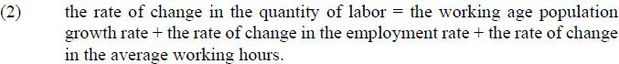
Meanwhile, the growth rate of labor quantity is the sum of the growth rate of the number of workers and the rate of change in the average working hours, and the former is in turn the sum of the growth rate of the working-age population and the rate of change in the employment rate. Thus, the labor quantity change is decomposed as follows:
Therefore, the effective labor input growth rate is decomposed into the working-age population growth rate, the rate of change in the employment rate, the rate of change in the average working hours, the effect of changes in education, and the effect of changes in the age structure of workers. Here, we will refer to the changes in working-age population growth and the age structure of workers as demographic factors, and the remainder (that is, changes in employment rate, working hours, and education) as quality-of-life-related choice factors.
Regarding the factors that affect labor productivity growth, we focus on structural change and the productivity catch-up effect (or changes in the advantage-of-backwardness effect), considering their relevance to economic development. Because the structural change effect only affects aggregate productivity, with the productivity of individual industries given,9 and the productivity catch-up effect is defined here as the effects on the productivity of individual industries, the two effects are independent of each other.
Therefore, the labor productivity growth rate is decomposed into the structural change effect, the advantage-of-backwardness effect, and a residual not explained by these two factors. As will be explained in Section IV, the structural change effect again consists of the Baumol effect and the Denison effect.
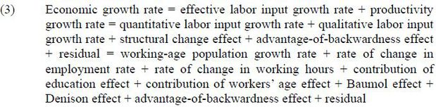
To summarize, the above decomposition can be expressed as the following equation (3):
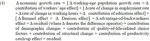
We reconstruct equation (3) according to the four categories of factors mentioned in the introduction and obtain equation (4).
Equations (3) and (4) are the decomposition equations of economic growth (or growth change) focusing on the developmental aspect of economic growth. Based on equation (4), we will estimate the contribution of each factor to the growth slowdown of the Korean economy.
We mainly use Korean data in this paper, as we investigate the Korean economy. The Korean data used in this paper are primarily those of the Bank of Korea (ECOS) and the National Statistical Office (Statistics Korea). Additionally, OECD, Conference Board, and Penn World Table 10.0 data were also used for some international comparisons.
First, the national account data of the Bank of Korea were used for Korea's GDP and value-added by industry. Data from the Economically Active Population Survey of the National Statistical Office (hereinafter referred to as “EAPS”) were used for the number of workers, working hours, the number of years of education, and the age composition of workers. Regarding the number of years of education and the age structure of workers, as only data on the overall industry average exist in EAPS, we assumed that education and the age of workers in each industry would be identical to the overall industry average. For working hours by industry, given that only data after 2000 exist in EAPS, we calculated pre-2000 working hours by industry from data on working hours by industry in 2000, the average working hours of the entire economy each year, and the number of workers by industry for each year. For this, we assumed that the annual rate of change of average working hours by industry before 2000 would be identical in all industries and calculated the common annual rate of change which makes, for example, the weighted average of the product of working hours by industry in 2000 and the common rate of change weighted by the number of workers by industry in 1999 equal to the average working hours of the entire economy in 1999. Although there is some time-series break in the data on the number of workers by industry in EAPS, because the difference is insignificant in the industry classification and in the time period covered in this study, these differences were disregarded.
In the estimation of the productivity catch-up effect, because an international comparison of productivity by industry is required, we used OECD STAN data, the Conference Board's international comparison data for manufacturing productivity, and Penn World Table data (PWT 10.0). For manufacturing productivity, the Conference Board data were mainly used as this dataset provides the longest time series. For productivity in other industries, OECD STAN data were used, and for labor quality (education) data, PWT data were used. A detailed explanation of the data used to estimate the productivity catch-up effect by industry is given in the appendix.
To examine the growth slowdown, it is necessary to compare the trend growth rates at two points in time. Here, we use a ten-year average growth rate as the trend growth rate. The HP filter seems inappropriate in our study due to its end point bias problem.
Given that this study addresses a growth slowdown, it would be better to compare the peak of the past growth trend or the trend growth rate just before the start of a significant slowdown with the most recent trend growth rate.
As of the time of the writing of this paper, data on the annual GDP of the Korean economy are available from 1953 to 2020 and data on the number of workers by industry are available from 1963 to 2020. Therefore, data for per-worker GDP exist from 1963 to 2020. Looking at the trend growth rate of per-worker GDP during this period, we find that it exhibits a pattern close to an inverted U-shape, peaking in the 1980s and then showing a downward trend (see Table 1). Based on the ten-year average growth rate, the per-worker GDP growth rate peaked (7.3 percent) between 1981 and 1991 and has since shown a downward trend. The per capita GDP growth rate was highest (9.2 percent) between 1967 and 1977 and second highest (9.1 percent) between 1981 and 1991 and has since been on the decline. For reference, the average growth rate from 1980 to 1990 is 8.7 percent in terms of per capita GDP and 7.0 percent in terms of per worker GDP. In short, both the per capita GDP growth rate and the per worker GDP growth rate peaked during the period from 1980 to the early 1990s and then continued to decline.
Note: * 1963~70 annual average growth rate.
Source: The Bank of Korea ECOS, National Statistical Office KOSIS.
Therefore, we compare the average growth rate of the period from 1980 to 1990 with a more recent trend growth rate. For the latter, we choose the average growth rate of the period from 2008 to 2018 for the following three reasons. First, 2020 can be regarded as an outlier in that during that year a severe economic recession occurred due to the COVID-19 pandemic. Second, in a similar context, the period from 2009 to 2019 is also inappropriate given that 2009 featured another recession due to the global financial crisis.10 Third, it was taken into account that most of the OECD, Conference Board, and PWT data include data up to 2018.
For starters, let us look at the quantitative labor input growth of Korea. As explained in the previous section, quantitative labor input growth is decomposed into the working-age population growth, the rate of change in the employment rate, and the rate of change in average working hours.
The annual growth rate of the working-age population in Korea exceeded 3 percent in the mid-1970s, but since then it has continued to decline. Korea currently has the lowest fertility rate in the world, and the working-age population is decreasing. The downward trend in the growth rate of the working-age population is due to the demographic transition, as explained in the introduction to this paper.
On the other hand, the employment rate in Korea continues to rise. The rise in the employment rate is mainly due to the rise of women's participation in economic activities. During the last forty years, the employment rate for women in Korea rose by about 20 percentage points. Meanwhile, average working hours in Korea are decreasing, and the speed of the decrease is accelerating.
Next, let us look at the qualitative change in labor input. As mentioned above, many empirical studies estimating qualitative changes in labor are based on Jacob Mincer's (1974) human capital earning function, which holds that differences in labor quality are reflected in wage differences in the labor market. This function is expressed in the form below,
where I, S, and X denote per hour earnings, education, and work experience, respectively.
In the estimation of equation (5), the number of years of education and the age of workers are used respectively as indicators of the education level and worker experience. We also follow this tradition and assume that the quality of labor is determined as in equation (6),
where S and X denote the number of years of education and the worker’s age, respectively.
First, for the specific functional form of ϕ , we follow the formula of Psacharopoulos (1994), which is also used in the Penn World Table. The equation presented by Psacharopoulos (1994) is shown below.
This equation reflects the empirical evidence that primary education makes a greater difference in the quality of work than higher education. In our estimation, S was obtained from data on the number of employed persons by level of education in the EAPS data.
On the other hand, regarding the functional form of ζ that reflects the skill level from age, there is no formula widely used among researchers, unlike in the case of education, and estimation results vary depending on the research.11 Here, we refer to the estimates of four previous studies with respect to ζ : Vollrath (2020), Heckman et al. (2003), Feyer (2008), and Aiyar et al. (2016).
Vollrath (2020) and Heckman et al. (2003) assume a quadratic functional form for ζ, following Mincer (1974). In the case of Vollrath (2020), equation (8) is presented for ζ.
The effective labor input (quality of labor) from experience is calculated as 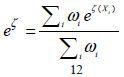 , where ωi denotes the proportion of age group i among all workers.12
Because the quadratic coefficient in equation (8) has a negative value, productivity (the quality of labor) decreases as workers age. In the case of estimation based on Heckman et al. (2003), we use the average of the estimates presented in Table 2 of the paper and take 0.107 and -0.0017 for the linear coefficient and the quadratic coefficient, respectively.13
Meanwhile, Feyer (2008) and Aiyar et al. (2016) used a method that directly estimates the relationship between the age group and productivity. Feyer (2008) found that workers in their 40s exhibited the highest productivity, and Aiyar et al. (2019) found that the greater the proportion of workers aged 55 and older, the lower the productivity, both suggesting that worker aging has a negative effect on productivity.14
Table 2 shows the contribution of changes in the age structure of the workforce to the Korean economy's effective labor input growth as calculated from the estimates of the four aforementioned studies. The contribution to growth slowdown is estimated to be between 0.1 and 0.9 percentage points. Among these estimates, we choose the estimate based on Vollrath (2020), which is the median value of the four estimates, and hereinafter use this value to represent the contribution of worker aging to the growth slowdown.
The trend of labor quality in the Korean economy from 1980 to 2018 as obtained from equations (6) to (8) shows that while the education effect has continued to increase, with the rate of increase slowing, the skill effect decreases after the 1990s, reflecting workforce aging (Korea is currently one of the most rapidly aging countries). Because the effect of skill (age) is smaller than that of education, the overall quality of labor, combining the two factors, shows an upward trend, with the rate of increase decelerating.
Multiplying the above estimate of qualitative change by the quantitative change yields the change in the total effective labor input. Table 3 summarizes the change in labor input growth for our analysis period. The rate of increase of effective labor inputs fell from an average of 4.1 percent in 1980 to 1990 to 0.3 percent between 2008 and 2018, a decrease of 3.8 percentage points during our analysis period. It is estimated that 1.6 percentage points can be attributed to the slowdown in the growth rate of the number of workers, 1.0 percentage points can be attributed to the reduction in working hours, and 1.1 percentage points can be attributed to the slowdown in the growth rate of labor quality (mainly due to the slowdown in the growth of education levels). The slowdown in the growth rate of the number of workers is almost entirely attributable to the slowdown in the growth of the working-age population. It appears that changes in the employment rate did not factor into the growth slowdown, as the employment rate has remained on an upward trend, similar to that in the high-growth era.
Table 4 is a reorganization of Table 3 according to the category of factors mentioned in equation (4). As shown in Table 4, the contribution of the demographic factors to the slowdown in total effective labor input growth is slightly larger than that of the quality-of-life-related choice factors. The division of changes in working hours into broad and narrow terms is due to the effect of changes in working hours caused by the structural change. Because there are considerably fewer working hours in the agricultural sector compared to those in other industries, the labor shift out of agriculture during industrialization has the effect of increasing the average working hours of the economy. ‘Working hours’ in a broad sense includes the effect of such a structural change, and ‘working hours’ in the narrow sense reflects only the change in working hours in individual industries, excluding the effect of the structural change.
Note: Figures for the employment rate and quality of labor represent the contributions to labor input growth.
Table 5 presents a comparison of the slowdowns in GDP growth and labor productivity growth. Approximately three-fifths of the slowdown in Korea’s economic growth during our analysis period is attributed to the slowdown in effective labor input growth, and approximately two-fifths is attributed to the slowdown in labor productivity growth. The discrepancy between the GDP growth rate and the sum of the growth rate of labor input and the growth rate of labor productivity is due to the calculation of the growth rate being based on discrete time.
The following equation represents the relationship between the economic growth rate and the growth rates of individual sectors:
Here, y denotes the economic growth rate and θi, yi, qi , and li represent the output share, output growth rate, labor productivity growth rate, and the labor input growth rate of sector i, respectively.
In equation (9), θi represents the real share of sector i when GDP is based on a fixed weight method, and the nominal share when GDP is based on a chain-weight method. After SNA93, the real GDP in most countries, including Korea, has been compiled using a chain-weight method. Hereinafter, we will discuss GDP with a chain-weight method in mind.
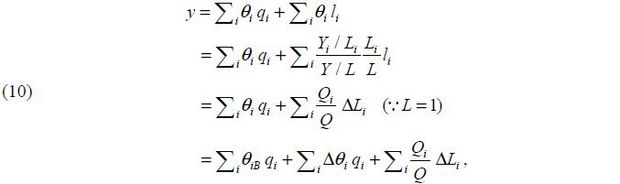
In Equation (9), if total labor input is fixed at 1, then y and li represent the growth rate of aggregate labor productivity and the rate of change in the employment (labor input) share of sector i, respectively. In this case, the following relationship is derived:
where θiB denotes θi at the base period, and Yi, Li, Qi and li represent the nominal output, employment share, nominal productivity level, and the growth rate of the employment share of sector i, respectively.
Structural change refers to the case where Δθi, ΔLi ≠ 0 in equation (10). We can see in equation (10) that if either qi (the productivity growth rate of sector i) or Qi (the nominal productivity level of sector i) is different for each sector,15 structural change causes a difference in the aggregate productivity growth rate. In other words, structural change affects the aggregate productivity growth rate through intersectoral differences in productivity growth rates or productivity levels. The second term of equation (10) refers to the effect of structural change on aggregate productivity growth through intersectoral differences in productivity growth rates, and the third term of equation (10) refers to the effect of structural change through intersectoral differences in nominal productivity levels. Following Nordhaus (2001), we refer to the former aspect as the Baumol effect and the latter aspect as the Denison effect. The scale or the sign of the Baumol effect or the Denison effect varies depending on the pattern of structural change and the patterns of intersectoral productivity differences.
Meanwhile, structural change and intersectoral productivity differences exhibit similar patterns in most countries. First, structural change due to industrialization exhibits a stylized pattern where the employment share of agriculture decreases, the share of services rises, and the share of manufacturing shows an inverted U-shaped change (see Figure 1 in Herrendorf et al. 2013). Second, the productivity level of agriculture tends to be significantly lower than those of the non-agricultural sectors. This phenomenon is presumed to stem from the facts that since agriculture is sensitive to seasonal and climatic factors, productivity is inevitably low for a considerable period of the year, and that the proportion of nonmarket production for self-consumption is relatively high in agriculture. Third, productivity growth in services tends to be significantly slower than in the goods-producing sectors. This seems to be due to the nature of the services sector, in which automation is relatively difficult and measuring quality improvements also poses challenges.
From these common patterns, we can expect that structural changes in most countries will affect economic growth in a similar fashion. First, the Denison effect will be positive during industrialization, and its size will vary according to the scale of the labor shift out of agriculture. Because the employment share of agriculture decreases with industrialization, the labor shift out of agriculture and accordingly the size of the Denison effect will increase at the initial stage of industrialization and decrease after a certain point. Second, the Baumol effect is likely to have a negative value, and this effect will appear more prominently during deindustrialization, when labor shifts to services from manufacturing as well as agriculture.
In general, since the Denison effect is much larger than the Baumol effect (in absolute value) in the early stage of industrialization, the effect of structural change on economic growth tends to have a positive value in the early stage of industrialization, decrease toward the latter stage of industrialization, and have a negative value in the deindustrialization stage.
The Korean economy also exhibits the same patterns of structural change and intersectoral productivity differences mentioned above. In the Korean economy, peak industrialization (the peak of the share of manufacturing employment) appeared in 1989. The share of agricultural employment fell from 63 percent in 1963 to 5 percent in 2018, the share of services employment increased from 25.8 percent to 69.8 percent in the same period, and the share of manufacturing employment rose from 7.9 percent in 1963 to 27.8 percent in 1989 before falling to 16.8 percent by 2018. Meanwhile, the patterns of the intersectoral productivity differences in Korea are shown in Table 6. In terms of per-worker nominal value-added, the productivity of agriculture is about a quarter of that of manufacturing, and less than half that of services. The real productivity growth rate of services is approximately half that of agriculture and manufacturing.
From equation (10) and considering the Korean data, we can estimate the effect of structural change on aggregate productivity growth. For this estimation, we divide the economy into four sectors: agriculture (including forestry and fisheries), manufacturing, services, and other sectors.16 The ‘other sectors’ include mining, utilities (electricity, gas, and water), and construction. Table 7 shows the estimation result of the Denison effect. (Because the Baumol effect is derived only as a comparison between two time points, as shown in equation (10), it cannot be demonstrated in the form shown in Table 7.) The ‘broad’ and the ‘narrow’ effects refer to effects with and without a change in average working hours due to structural change, respectively. The (broad) Denison effect in the Korean economy reached an average of 1.2 to 1.4 percentage points per year in the 1970s and 1980s, demonstrating its contribution to Korea’s high growth. On the other hand, the Denison effect in the 2010s was almost zero, suggesting that (the change in) the Denison effect also played an important role in the growth slowdown after the end of high growth.
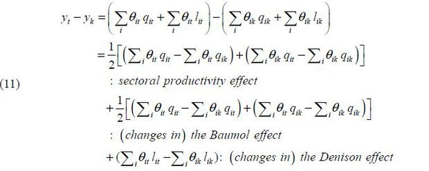
Next, let us look at the contribution of the effect of structural change to the growth slowdown during our analysis period. Equation (11) can be derived from Equation (10) to estimate the contribution of structural change to the change in the aggregate productivity growth rate between two points in time.
That is, the change in the aggregate productivity growth rate between two time points, t and k, can be decomposed into (the change in) the Baumol effect, (the change in) the Denison effect, and the effect of changes in sectoral productivity growth rates. In our case, because we compare average growth rates for the years 1980-90 and 2008-18—not single-year growth rates—the two sides of the equation above do not match exactly but are instead approximated with some errors (the discrepancy is no greater than 0.1 percentage points).
We used the arithmetic mean of the 2008 nominal share and the 2017 nominal share  for θit and the arithmetic mean of the 1980 nominal share and the 1989 nominal share
  for θik in the estimation of equation (11). Given that the Denison effect can be estimated
annually, the average of the annual Denison effect for the period was used (e.g.,
the Denison effect for the period from 1980 to 1990 is the average of the Denison
effect for each year from 1980 to 1990).
for θik in the estimation of equation (11). Given that the Denison effect can be estimated
annually, the average of the annual Denison effect for the period was used (e.g.,
the Denison effect for the period from 1980 to 1990 is the average of the Denison
effect for each year from 1980 to 1990).
The results estimated in this way are shown in Table 8. For per worker productivity (upper table in Table 8), the contribution of (broad) structural change to the growth slowdown is 1.3 percentage points per year on average, which explains approximately 26 percent of the slowdown in aggregate productivity growth during our analysis period. For effective labor productivity, the contribution of (narrow) structural change to the growth slowdown is 0.9 percentage points per year on average, which explains approximately 36 percent of the slowdown in aggregate productivity growth. In both cases, the contribution of the Denison effect is much greater than that of the Baumol effect.17
As shown in equation (11), the portion of the change in the aggregate productivity growth rate that is not explained by the structural change effect is caused by the change in the productivity growth rates of individual sectors. When productivity growth rates in several industries show a declining trend, a productivity catch-up effect based on the ‘advantage of backwardness’ can be seen as one of the most likely causes, particularly in latecomer industrializers such as Korea.
In this section, we estimate the contribution of the productivity catch-up effect to the slowdowns in sectoral productivity growth and economic growth in the Korean economy. The industries to be analyzed are agriculture, manufacturing, and services, as examined in the previous section. The ‘other industries’ category is excluded from the estimation, as these industries are composed of sectors with different characteristics and account for only a small proportion of the total economy in Korea. We estimate the productivity catch-up effect in the aforementioned three sectors and then calculate the contribution of the productivity catch-up effect to the slowdown in economic growth based on the assumption that the proportion of the contribution of the effects of the three sectors to the slowdown of the three-sector aggregate productivity growth is identical to the proportion of the contribution of the productivity catch-up effect to the slowdown of aggregate productivity growth of the entire economy.
Specifically, we estimate the effect here based on the convergence equation derived from the technology diffusion (or technology leader/follower) model. This model explains the tendency of technology followers to grow faster than technology leaders based on the fact that imitation costs less than innovation. However, if the productivity of a follower catches up to that of the leader, there is less room for imitation; consequently, the follower’s productivity growth rate slows and ultimately converges to that of the leader. From this logic, the following convergence equation is derived:18
where qi and Qi denote the productivity growth rate and productivity level of a follower country
i, respectively, q1 and Q1 denote the productivity growth rate and productivity level of a leading country,
respectively, and  denotes
  in a steady state.
Assuming that  is constant, we can calculate the productivity catch-up effect by estimating 𝜇 in
equation (12).
is constant, we can calculate the productivity catch-up effect by estimating 𝜇 in
equation (12).
From equation (12), we obtain
Because gi is the growth rate of  , we also obtain from equation (13)
Taking the logarithm of both sides of equation (14), we obtain
Therefore,
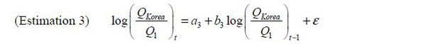
We can also estimate μ from equation (16). While in a conventional convergence estimation, the goal is to estimate the speed of convergence common to many countries, the purpose of our estimation is to estimate the speed of convergence of Korean industries. Thus, if possible, it would be meaningful to estimate the convergence speed based only on Korean data. Because equation (16) uses the relative productivity level, which is much less volatile than the growth rate, significant estimation results can be obtained using annual data instead of the five- or ten-year average data generally used in convergence estimations based on growth rate data. Therefore, we can estimate equation (16) with Korean annual productivity data.
Here, we estimate μ from the following four equations:
While Estimations 3 and 4 are based on equation (16), in Estimation 4, the change in Korea’s unemployment rate from the previous year was added as an explanatory variable to control the effects of business cycles. We used the farmhouse unemployment rate for agriculture and the unemployment rate of the entire economy for manufacturing and services.
In Estimations 1 and 2, the values obtained by multiplying the regression coefficients ( b1 and b2 ) by (-1) correspond to the estimated value of μ in equation (12), and in Estimations 3 and 4, the values of (1- bi ) correspond to the estimated value of μ .19 The coefficients b1 and b2 are expected to have negative values, b3 and b4 are expected to have positive values of less than 1, and c1 and c2 are expected to have a positive value and a negative value, respectively. In Estimations 1 and 2, we used the panel fixed effect model20 based on multi-country panel data and used a five-year average growth rate for the productivity growth rate. Estimations 3 and 4 were estimated with an autoregressive model using annual data from 1970 to 2018 on Korea’s relative productivity level compared to a technology leader.
US industries were assumed to be the technology leader in all three industries. For manufacturing, Conference Board data were used, as these data provide the longest time series that is internationally comparable, and for agriculture and services, OECD STAN data were used. Countries where the time series were too short, some data did not exist, or no catch-up phenomenon was observed were excluded. For the exchange rate to compare productivity levels, we used the market exchange rate for manufacturing and agriculture and the purchasing power parity exchange rate for services, which are mainly non-tradable. Details of the data used for the estimation are explained in Appendix 1.
The results of Estimations 1 to 4 are shown in the tables in Appendix 2. Table 9 summarizes the estimated μ values ( ) obtained from the estimation results. For reference, Rodrik (2012) estimated the convergence coefficient for manufacturing productivity using methods
similar to ours, and the estimated coefficients were 1.6 (unconditional convergence:
a model without a country fixed effect) to 6.0 (conditional convergence: a model with
a country fixed effect). Our for manufacturing (1.9 to 5.8) is not much different from Rodrik’s estimates.
) obtained from the estimation results. For reference, Rodrik (2012) estimated the convergence coefficient for manufacturing productivity using methods
similar to ours, and the estimated coefficients were 1.6 (unconditional convergence:
a model without a country fixed effect) to 6.0 (conditional convergence: a model with
a country fixed effect). Our for manufacturing (1.9 to 5.8) is not much different from Rodrik’s estimates.
We take the smaller of the actual slowdown and the value obtained from equation (12)
and in Table 9 as the productivity catch-up effect, as in equation (17).21
The effect of catch-up on the productivity growth slowdown in sector i between period t and k
where QKorea,i,t and qit denote the productivity level and the productivity growth rate of Korean sector i at period t, respectively, and Q1i,t denotes the productivity level of US sector i.
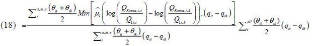
The contribution of the productivity catch-up effect to the aggregate productivity growth slowdown between periods t and k is obtained from equation (18).
Productivity catch-up effect on the aggregate productivity growth slowdown between t and k
where a, m, and s represent agriculture, manufacturing and services, respectively.
The productivity catch-up effects between 1980-90 and 2008-18 obtained in this way are summarized in Table 10. It is estimated that the productivity catch-up effect contributed between 0.82 and 1.65 percentage points to the slowdown in aggregate productivity growth in Korea between 1980-90 and 2008-18.
According to our estimations in Sections IV and V, approximately 0.9 percentage points of the 2.7 percentage-point slowdown in productivity growth between 1980-90 and 2008-18 can be attributed to structural change (narrow), and 0.8 to 1.7 percentage points can be attributed to the productivity catch-up effect. Therefore, the slowdown in productivity growth of Korea that is not explained by these two factors is 0.1 to 1.0 percentage points. A decrease in innovation or reduced efficiency may have caused this unexplained productivity slowdown.
Meanwhile, we know that the productivity growth rate decreased not only in Korea but also in most advanced countries during our analysis period. For convenience, let us call this the global productivity slowdown. The global productivity slowdown could be a result of a slowdown in the pace of global technological progress in related industries. Thus, it is highly likely that the global productivity slowdown has also affected the productivity growth rate of Korean industries. However, because in the estimation of the productivity catch-up effect we estimated the changes in the effect of the advantage of backwardness, or the changes in relative productivity growth rates of Korean industries compared to the technology leader, this aspect may not be properly reflected in the estimation in Section V. Accordingly, we can presume that part of the unexplained productivity slowdown mentioned above may be due to the global productivity slowdown.
In this case, it is difficult to know how much the global productivity slowdown has affected the industrial productivity slowdown in Korea. However, as a reference indicator, we can examine how much change in the aggregate productivity growth rate of Korea would appear if Korean industries had experienced the same slowdown in the productivity growth rate as the corresponding industries in the technology leader country. This is, so to speak, an estimate of the slowdown in economic growth assuming that the global productivity slowdown would have had an equal impact on the productivity growth rate of the corresponding industry in Korea. This value can be calculated from the industrial structure of Korea and the magnitude of the productivity growth slowdown by sector in the technology leader. The estimate is 0.8 percentage points in the case of the US as the technology leader and 1.5 percentage points if using the average of G7 countries as the technology leader.22
Table 11 summarizes the results of our analyses in Sections III to VI. As shown in the table, the four categories of factors we investigated account for between 85 and 98 percent of the growth slowdown. In other words, most of the slowdown in Korea’s GDP growth over the past thirty years can be attributed to demographic changes (the slowdown in population growth and aging of the labor force), the accelerated reduction in working hours, the slowdown in the extension of education, the effect of the structural change, and productivity catch-up effects in major industries. Among the four categories of factors, the demographic factor accounts for approximately 32 percent of the growth slowdown, with each of the other three factors (quality-of-life-related choice factors, structural change, and productivity catch-up effect) accounting for approximately 20 percent. Only 2 to 15 percent of the growth slowdown is not accounted for by these four categories of factors. In addition, considering the effect of the global productivity slowdown mentioned in Section VI, it appears that proportion of the growth slowdown not explained by the factors considered here is very small.
Note: *based on US productivity.
** based on G7 productivity.
These estimation results suggest that the growth slowdown of the Korean economy is basically a consequence of its successful economic development,23 or a case of rapid convergence. In other words, our estimates do not support the growth crisis hypothesis that Korea’s growth slowdown is mainly the result of failures in innovation or policies.24
Some of the developmental factors that we examined as the causes of the slowdown in economic growth are those that themselves exhibited a growth slowdown or a decreasing trend during our analysis period. This suggests that the same factors before such a slowdown or a decreasing trend may have played an important role in the Korean high growth as well.
Such factors will include high population growth in the early phase of the demographic transition, a substantial rise in women’s employment rate, a rapid increase in years of education, a large Denison effect due to the compressed industrialization, and high growth of industrial productivity owing to the advantage of backwardness. Using equation (3) explained in Section II, we examined the contribution of these factors to the Korean economic growth from 1980 to 1990, the peak of the high growth period. Table 12 summarizes the results.25
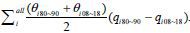
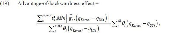
Some explanation will be necessary concerning the method used to estimate the productivity growth effect due to the advantage of backwardness (H in Table 12). Although the estimation here also uses the model and the regression results from Section V, while we estimated the change in the effect of the advantage of backwardness during our analysis period in Section V, we estimate here the average size of the effect of the advantage of backwardness in the period from 1980 to 1990. The size of the effect of the advantage of backwardness is regarded as the estimated relative productivity growth rates of Korean industries compared to US industries (that is, the estimated differences in industrial productivity growth rates between two countries) when Korean industries’ productivity levels relative to those of US industries are given. For relative productivity levels, a ten-year average (1980 to 1989) was used, and by substituting the relative productivity levels and the estimated coefficient values into each estimation equation, estimates of Korean industries’ relative productivity growth rates were obtained. For Estimations 1 and 2, estimated values of the Korean dummy coefficients were also applied. As in Section V, the smaller of the estimated result and the actual productivity growth rate gap between Korean industries and US industries was adopted as the sectoral ‘advantage of backwardness’ effect, and the aggregate effect was obtained by equation (19) below, similarly to equation (18) in Section V.
Notes: * Figure based on US productivity.
** Figure based on G7 average productivity.
*** Discrepancy due to growth rate based on discrete time.
Where  denotes the estimated relative productivity growth rate in Korean sector i.
As shown in Table 12, during the high growth of the Korean economy from 1980 to 1990, about 70 percent of the growth is accounted for by the five developmental factors mentioned above. Add to this the average productivity growth rate of the technology leader (designated as the ‘world productivity growth rate’ in the eleventh row of Table 12),26 and the five developmental factors and world productivity growth account for about 90 percent of Korea’s high growth during this period.
The high growth of East Asian countries, including Korea, was called the Asian miracle. However, if a miracle refers to a phenomenon that is difficult to explain, according to the estimation results above, Korea’s high growth was not a miracle. The estimation above demonstrates that Korea’s relatively high growth compared to the growth in other economies can also be mostly explained by developmental factors27 — that is, it was made possible by factors that are likely to appear at a specific stage of economic development and have a temporary nature. The rapid increases in populations, years of education, and women’s employment rate, the large Denison effect, and the advantage-of-backwardness effect are all unsustainable, and most of them (growth rates or levels) are bound to converge to zero. Thus, it can be said that the factors that made high growth possible also made the subsequent large growth slowdown inevitable.
In this study, we have demonstrated that the growth slowdown of the Korean economy over the past thirty years is mostly explained by factors associated with economic development, and that the high growth of the 1980s can also be largely attributed to the same factors. This suggests that Korea’s high growth and the subsequent large slowdown in growth can basically be regarded as a single process of a rapid convergence or a rapid catch-up.
The contribution of this study is in its empirical and methodological aspects. This study defines the role of developmental factors in Korea’s growth slowdown through an estimation of their contributions, thus providing a different perspective from previous studies mainly based on growth accounting. In terms of methodology, decomposition of economic growth focusing on developmental factors or estimation methods of the effects of structural change can be seen as new attempts.
Although this study focuses on the Korean economy, because the factors examined here exhibit similar patterns of change over the course of economic development of most countries, we think that the estimation results of this study can have more general implications. The acceleration and deceleration of economic growth and the role of developmental factors in these growth changes, as found in Korea’s economic development experience, are highly likely to appear with similar patterns in the economic development of many countries. Indeed, the long-term economic growth of East Asian countries shows distinct temporal patterns that are similar to each other.28 Similar patterns are also observed in many other economies, albeit with some differences in scale.29
Studies of the relationship between economic growth and economic development can broaden our understanding of long-term growth changes and help predict future growth in industrializing economies. As more latecomers are industrialized and their experiences accumulate, more empirical studies will be possible. The estimation results and methodology used here can provide a reference for such studies.
We used manufacturing productivity data from the Conference Board to estimate the productivity catch-up effect in manufacturing. This source provides data on nominal and real value-added, the number of workers, average working hours, and exchange rates by country from 1950 to 2018 (the length of the time series varies from country to country). Given that we wanted to estimate labor productivity in an efficiency unit, we additionally used education (human capital) data provided by PWT 10.0. Education data in PWT are only the average of the overall economy, and there are no sectoral data; therefore, the same data were applied to all industries. While a five-year average growth rate was used for the productivity growth rate, because the last period ends in 2018, a three-year average growth rate was used for 2015 to 2018. The relative (nominal) productivity level was obtained from the value of the first year of the five-year average growth rate; i.e., the productivity growth rate of 1950 to 1955 corresponds to the relative productivity level of 1950 in the regression analysis. Countries were selected with the criteria that the variables required for analysis exist for at least 20 years and a significant productivity catch-up (significant upward trend in the productivity level relative to that of the US) is observed. The selected countries were Korea, the USA, Australia, Austria, Belgium, Brazil, Canada, Denmark, Finland, France, Germany, Greece, Ireland, Italy, Japan, Mexico, Netherlands, Norway, Portugal, Singapore, Spain, Sweden, the UK, and Taiwan, for a total of 24 countries.
OECD STAN data (ISIC rev.4, SNA 08, 2020 ed.) were used for agriculture and services. These data provide statistics on nominal and real value-added, the number of workers, and working hours from 1970 to 2019 (the length of the time series varies from country to country). Because data from the United States, which we assume to be the technology leader, are available until 2018, we used only data up to 2018. In many countries, the time series for working hours by industry in the STAN DB is either very short or not available. However, as time-series and cross-country comparisons of productivity are required, it is necessary to secure as long a time series as possible while applying the same criterion for each country. Considering this problem and the fact that long time-series data are available for most countries for average working hours in the overall economy, we applied data on average working hours in the overall economy to both agriculture and services. The method of calculating the effective labor input, the productivity growth rate or relative productivity level is identical to that of manufacturing. The sample criteria are the same as those used for manufacturing. The selected countries were Korea, the USA, Australia, Austria, Belgium, Denmark, Finland, France, Germany, Greece, Ireland, Italy, Japan, Luxembourg, Mexico, Netherlands, New Zealand, Norway, Portugal, Spain, Sweden, Switzerland, and the UK, for a total of 23 countries.
Studies focusing on growth slowdowns in high-growth economies include the following. First, Eichengreen et al. (2012a, 2012b, and 2016) examined the relationship between growth slowdowns and income levels. They did not investigate the causes of the growth slowdown, but they pointed out that the slowdown is highly correlated with several factors such as the demographic structure, consumption rate, exchange rate, education level, and product structure of exports. Next, regarding studies of the growth slowdown in the Japanese economy, Yoshikawa (1992) examined the end of high growth in the 1970s, and Hayashi and Prescott (2003) investigated the causes of the slowdown in the 1990s. The causes of the slowdown were discussed in terms of a Lewis turning point and the maturation of durable goods consumption in Yoshikawa (1992) and in terms of the slowdown in TFP growth in Hayashi and Prescott (2003). As for studies of Korea’s growth slowdown, Han and Shin (2008) and Seok and Lee (2021) examined the causes of the slowdown using growth accounting, while Eichengreen et al. (2012) and Han and Lee (2020) also analyzed Korean economic growth mainly through growth accounting, taking into account the slowdown. Kang (2001 and 2009) investigated the role of structural change during the 1990s slowdown, and Kim (2016) argued that stagnation of human capital and technological progress were the causes of the growth slowdown. On the other hand, although not focusing on high-growth economies, there are studies of productivity slowdowns of advanced economies in the 1970s (Maddison 1987, Nordhaus 2004), studies of the US growth slowdown (Gordon 2016, Antolin-Diaz et al, 2016), and theoretical studies deriving the possibility of a long-term growth slowdown from multi-sector models (Baumol 1967, Echevarria 1997, and Duernecker et al. 2021). Convergence is also linked to growth slowdowns, but it appears that this subject is approached more often from the perspective of cross-sectional differences in economic growth than from the perspective of temporal changes in economic growth.
The reason for choosing this method and the specifics of our analysis method will be explained in Section II-A.
According to Smil (2019), “the demographic transition was conceptualized by Warren Thompson (1929), called first a “demographic transition” by Landry (1934), and received its standard formulations from Notestein (1945) and Davis (1945).” (Smil (2019), p.317.)
As will be explained in Section II-C, we investigate the growth slowdown by comparing the average growth from 1980 to 1990 with the average growth from 2008 to 2018. Korea’s economic growth rate slowed from an annual average of 10 percent in the 1980s to an annual average of 3.2 percent from 2008 to 2018. During the same period, the labor input growth rate slowed from 4.1 percent to 0.3 percent, capital input slowed from 11.4 percent to 3.8 percent, and the TFP growth rate fell from 2.6 percent to 1.2 percent. Labor input is based on efficiency units, and the estimation method is explained in Section III. For capital input, Bank of Korea data on productive capital stock was used. For the factor income share used in calculating TFP, Bank of Korea data on domestic factor income was used. The factor income share was obtained excluding mixed income, and for years in which there is no mixed income data, mixed income was estimated by applying the ratio of mixed income to household operating surplus for the nearest year for which data exist.
Since “growth accounting treats all capital formation as a wholly exogenous explanatory factor, it tends to overstate the role of capital and understate the role of innovation in the growth process” (Hulten 2000, p.34). See also “Limitations of Growth Accounting” in Barro and Sala-i-Martin (1995), p.352. Rhymes (1971) and Hulten (1975) also addressed the same issue. This underestimation problem can be more serious in the case of East Asian high growth, where capital growth rate and capital income share are significantly higher than other economies. For example, according to Hulten and Srinivasan (1999), the growth contribution of technological progress in East Asian growth is estimated to be 1.5 times larger when assuming Harrod neutral technological progress than the conventional TFP estimation assuming Hicks neutral technological progress.
Unlike labor, because capital is “a produced factor of production” (Samuelson and Nordhaus (2005), p.33), it
Kaldor’s stylized facts of economic growth and steady-state growth are compatible with Harrod-neutral technological progress, not Hicks-neutral technological progress.
The Korean economy showed a sharp drop in its growth rate in 2009 due to the impact of the global financial crisis and the Great Recession, rebounding sharply in 2010 and regaining the previous trend. (While Korea’s average annual growth rate between 2000 and 2010 was 4.7 percent, the economic growth rate was 0.8 percent in 2009 and 6.8 percent in 2010.) Therefore, the average annual growth rate for 2009~19 is highly likely to overestimate the trend growth rate, as the base year 2009 was a year of severe economic recession.
For example, work by Murphy and Welch (1990) argues that a quartic function fits the data better than Mincer's quadratic function. Meanwhile, Burtless (2013) maintains that there is little evidence that aging has hurt productivity, unlike other studies mentioned here.
We used data for ten age groups in the EAPS data, with the midpoint age of each group used as 𝑋i.
Heckman et al. (2003) provides 12 estimates (6 for US whites and 6 for blacks) based on six decennial census datasets from 1940 to 1990. We used the average of 12 estimates.
We used the estimates in column 1 of Table 1 in Feyer (2008). With regard to Aiyar (2016), we used the sum of capital deepening estimates and the TFP estimates in Table 4 of the paper.
If wages are identical across industries and relative prices are determined by the unit labor cost, then the inter-industry ratio of nominal productivity remains constant.
In general, the more subdivided the industry classification, the more precisely the effect of structural change can be estimated. However, the more detailed the industry classification, the greater the data constraints and the higher the complexity of the analysis. In this regard, there is a tradeoff relationship between the precision of estimation results and the cost of estimation, and the level of industry classification should be selected considering this relationship. There are two main reasons for selecting the industry classification used in this study to estimate the structural change effect. First, the industry classification adopted in this study is conventionally used in studies dealing with structural change, and we followed this practice. Second, and more importantly, we are interested in a specific structural change in this study, not all structural changes. Given that the purpose of this study is to examine the role of developmental factors in the growth slowdown of the Korean economy, we are interested in only structural changes with clear developmental implications. In other words, the object of our analysis is such structural changes that appear generally in the process of the economic development of most countries and have stylized patterns. Previous studies and data show that such structural changes are observed at the same level of industry classification as ours.
Unlike this case of Korea, the Baumol effect is greater than the Denison effect in terms of absolute value in countries where deindustrialization has progressed significantly, such as the present-day US.
Because percentage values were used for the growth rates in Estimations 1 and 2, in the case of Estimations 3 and 4, strictly speaking, (1 − 𝑏i) × 100 corresponds to μ.
Given that we want to estimate the convergence speed of Korean industries, we used a model with a country ixed effect. However, according to Barro (2012), the convergence coefficient tends to be overestimated with Hurwicz-Nickell bias when using a model with a country fixed effect and data with short time series.
As shown in Table 10, in the services sector, in which the scale of the growth slowdown was relatively small during our analysis period, all estimation results were larger than the actual slowdown. Hence, we used the actual slowdown as the catch-up effect.
The slowdown in productivity growth was examined for six sectors (agriculture, manufacturing, services, mining, utility, and construction), and the Korean industrial structure was calculated from the average of the sectoral share of nominal value-added in 1980 and 2017.
Korea after the mid-20th century is the most representative example of successful economic development. In 2021, UNCTAD changed Korea's status from a developing country to a developed country, the first time it had done so for a country in its 57-year history. In the aftermath of the Korean War, Korea was one of the poorest countries in the world, but it has surpassed the UK, Italy, and Japan in per adult PPP income, according to World Inequality Report 2022.
Other evidence not consistent with the growth crisis hypothesis is that Korea’s productivity growth rate is still significantly higher than those of other developed countries, despite the fact that its productivity level is close to those of major developed countries. While Korea’s per hour GDP level in 2018 (based on the market exchange rate) is 68 percent of the average of G7 excluding the US, Korea’s average annual per-hour GDP growth rate between 2008 and 2018 (3.0 percent) is about five times higher than the corresponding G7 average, excluding the US (0.6 percent).
Because the contributions of changes in working hours, the worker age effect, and the Baumol effect are negligible, they are omitted in Table 12.
The world productivity growth rate was obtained by applying the productivity growth rate of six industries in the US or G7 countries and Korea’s industrial structure in the 1980s, as in the estimation of the global productivity slowdown in Section VI.
Of course, not all countries that have undergone the same economic development process show compressed industrialization or economic growth as fast as those in Korea. In that sense, high growth is also a phenomenon with cross-sectional specificity. In order to understand East Asian high growth properly, both the temporal and cross-sectional characteristics need to be explained. However, it seems methodologically desirable to approach these two issues separately. The discussion in this paper is about the former.
For instance, both Japan and Taiwan exhibit patterns of high growth followed by subsequent periods of slowdown, similar to that of the Korean economy. Referring to data from PWT 10.0, Japan experienced an average annual economic growth rate of 9.2 percent during its high-growth era (1955-73), subsequently slowing to 0.6 percent between 2008 and 2018. Similarly, Taiwan’s economic growth rate decreased from 9.6 percent in the high-growth phase (1960-90) to 3.1 percent between 2008 and 2018.
Based on the GGDC (Groningen Growth and Development Center) 10-Sector Database, the Penn World Table, Maddison project data, and long-term productivity data from Bergeaud et al. (2016), Kang and Park (2019) demonstrates that the long-term per-worker GDP growth trends of major industrialized economies exhibit patterns similar to an inverted U-shape, and their peak growths tend to appear close to peak industrializations in terms of timing.
, & . (1992, April). Convergence. Journal of Political Economy, 100, 223-251, https://doi.org/10.1086/261816.
(1945). The World Demographic Transition. Annals of the American Academy of Political and Social Science, 237, 1-11, https://doi.org/10.1177/000271624523700102.
(1997). Changes in Sectoral Composition Associated with Economic Growth. International Economic Review, 38, 431-452, https://doi.org/10.2307/2527382.
, , & (2012a). When Fast Growing Economies Slow Down: International Evidence and Implications for China. Asian Economic Papers, 11(1), 42-87, https://doi.org/10.1162/ASEP_a_00118.
, & (1990). Empirical Age-Earnings Profiles. Journal of Labor Economics, 8(2), 202-229, https://doi.org/10.1086/298220.
(1994). Returns to Investment in Education: A Global Update. World Development, 22(9), 1325-1343, https://doi.org/10.1016/0305-750X(94)90007-8.
(1929). Population. American Journal of Sociology, 34, 959-975, https://doi.org/10.1086/214874.