- P-ISSN 2586-2995
- E-ISSN 2586-4130

This paper studies how COVID-19 has affected the labor market in Korea through a general equilibrium model with multiple industries and occupations. In the model, workers are allocated to one of many occupations in an industry, and industrial or occupational shocks alter the employment structure. I calibrate the model with Korean data and identify industrial and occupational shocks, referred to here as COVID-19 shocks, behind the employment dynamics in 2020 and 2021. I find that COVID-19 shocks are more severe for those with jobs with a higher risk of infection and in those that are more difficult to do from home. Interestingly, the relationship between COVID-19 shocks and infection risk weakened as the pandemic progressed, whereas the relationship between COVID-19 shocks and easiness of work-from-home strengthened. I interpret the results as meaning that the pandemic may direct future technological changes to replace tasks that require contact-intensive steps, and I simulate the impact of such technological changes through the lens of the model. The results show that such technological changes will lower the demand for manual workers compared to the demands for other occupations. This contrasts with the earlier trend of job polarization, where manual workers continued to increase their employment share, with the share of routine workers secularly declining at the same time.
COVID-19, Contact Intensiveness, Job Polarization, Directed Technological Change
E24, I14, J23, O33
COVID-19 has led the world economy to the worst economic crisis since the Great Depression. The IMF’s World Economic Outlook estimates a -3.1% drop in global GDP in 2020, a much more severe recession than the -0.1% drop in global GDP during the Global Financial Crisis. The labor market was hit especially hard by the spread of the virus. COVID-19 dampened labor demand and reduced the labor supply due to quarantine policies and fear of infection. In Korea, the number of employed persons decreased by 1.8% (473 thousands persons) from February of 2020 to February of 2021.
The economic impact of the pandemic may not be confined to a short-term recession. Structural changes in the labor market were underway even before the pandemic, and these changes continued intensively during the economic recession. Many studies have documented a declining trend of middle-skill routine worker employment (as opposed to high-skill cognitive workers and low-skill manual workers) over several decades, a phenomenon referred to as job polarization. This disappearance of middle-skill jobs has also been more prominent during economic recessions as compared to normal times (Jaimovich and Siu, 2020). The recent recession with the COVID-19 pandemic, not an exception, could also accelerate structural changes in the labor market.
The pandemic appears to affect not only the speed but also the direction of structural changes in the labor market. The COVID-19 recession has had significantly heterogeneous impacts across industries and occupations compared to previous recessions (Aum, Lee, and Shin, 2021a). The heterogeneous nature of the COVID-19 shock implies that relative productivity levels between occupations and industries must have diverged to a substantial extent during the pandemic, likely affecting the direction of technological change. Therefore, as researchers grope for the direction of change in the labor market structure after the COVID-19 pandemic, analyses of the nature of shocks that stand out during the pandemic are necessary.
This paper aims to identify COVID-19 shocks that differ across industries and occupations during the pandemic, thereby deriving implications pertaining to the post-COVID-19 labor market structure. To this end, I introduce a general equilibrium model with multiple industries and occupations in which agents are allocated to one of many occupations in one of many industries. Each industry employs all occupations but with different intensities, and hence both industry- and occupation-specific shocks alter the industrial and occupational employment structures simultaneously. For example, when an occupational shock hits service jobs, it affects the industrial structure as well because the fraction of service jobs differs across industries. The model suitably captures structural changes in the labor market before the pandemic and hence enables us to compare past trends and future changes within a single framework.
I calibrate the model based on Korean data in 2019, just prior to the pandemic, after which I estimate the industrial and occupational productivity shocks that generate Korea’s employment dynamics in 2020 and 2021. To examine the characteristics of the identified shocks, I check whether and how the shocks correlate with the infection risk or the easiness of work from home by industry and occupation. The results are mainly twofold.
First, during the pandemic, employment was hit harder in industries and occupations with higher infection risks and/or difficulties in work from home. In particular, the easiness of work from home was more closely linked to occupational shocks than industrial shocks, implying that it is crucial to pay particular attention to occupational heterogeneity to understand employment dynamics in Korea.
Second, the relationship between employment shocks and the infection risk or easiness of work from home varies over time. In 2020, when employment fell rapidly due to the spread of COVID-19, only the risk of infection showed a significant correlation with COVID-19 shocks. However, in 2021, when employment began gradually to recover, the correlation with easiness of work from home became more significant, whereas the correlation with the risk of infection weakened. This result seems to indicate that the risk of infection was important in the earlier stage of the pandemic, whereas easiness of work-from-home gradually came to eclipse the risk of infection as the pandemic progressed. In this regard, I consider that the effect of infection risk is transitory, while the effect of easiness of work-from-home is more structural and of the type of effect to which technology responds. That is, the cost of contact-intensive tasks rose sharply during the pandemic, especially in its later stage, inducing technological progress to replace such tasks. Recent technological changes have already made the replacement of contact-intensive tasks feasible, as seen in telemedicine, smart finance, and online education platforms. The rapid growth of the online-to-offline (O2O) market before and during the pandemic also suggests that replacing contact-intensive tasks is feasible to some extent. These incentives and the feasibility issue indicate the possibility that technological changes will accelerate the replacement of contact-intensive tasks in the future.
Against this backdrop, I utilize the model to quantify the impacts of the Contact-intensive task Biased Technological Changes (henceforth CBTC) on employment structures in the future, though accurately predicting the future direction of technological change is not possible. Specifically, I compare the employment structure over the next five years with and without CBTC as measured based on each occupation’s easiness of work from home. Note that CBTC in this paper would have distinct implications on the labor market structure from Routine Biased Technological Change (henceforth RBTC), a widely accepted view in the recent literature before the pandemic. Jobs have been polarized at least since 1980, and the polarization of the labor market has been often linked to the effect of RBTC (Autor, Levy, and Murnane, 2003, Autor and Dorn, 2013, among others). Specifically, the RBTC hypothesis argued that the rapid evolution of IT technology has displaced jobs that mainly involve routine tasks, which are mostly middle-wage jobs. At the same time, RBTC raised the demand for both low-wage manual workers and high-wage cognitive workers, leading to the disappearance of middle-skill routine jobs.
The simulation results in this paper confirm that CBTC has a different impact on the labor market structure from RBTC. Specifically, CBTC reduces the demand for manual workers compared to the pre-COVID-19 trend. Accordingly, due to CBTC, the decline of routine workers is eased and the demand for cognitive workers becomes stronger compared to the earlier trend. This result contrasts with the significant increase in manual employment, accompanied by the decline in routine employment before the pandemic, i.e., job polarization driven by RBTC. An example that can illustrate the different impacts of CBTC from RBTC is the widespread use of kiosks in restaurants during the pandemic. Kiosks not only automate the routine receipt of food orders but also reduce face-to-face contact between customers and workers. In the view of my analysis, this type of automation differs from the automation of an assembly process in a manufacturing plant, which only replaces routine tasks.
The remainder of the paper is as follows. Section 2 introduces the model. In Section 3, I set the parameter values of the model based on Korean data. Section 4 identifies and examines the characteristics of structural shocks by industry and occupation ultimately to explain the labor market in 2020 and 2021. Section 5 discusses implications related to structural changes in the post-COVID-19 labor market if technological changes continue to replace contact-intensive tasks in the coming years. Section 6 concludes the paper.
The model here is a multi-sector macroeconomic model similar to that of Aum, Lee, and Shin (2018). Different from Aum, Lee, and Shin (2018), I do not distinguish between different types of capital goods, instead stressing the endogenous allocation of labor into both industry and occupation. The endogenous determination of the industrial and occupational structure enables an analysis of structural changes both in an occupational dimension and an industrial dimension. There are at least two reasons why I focus on both industrial and occupational dimensions simultaneously.
First, because the labor market has undergone structural changes before the pandemic, it is necessary to take past trends into account for a clear understanding of how the post-pandemic labor market structure would be different with and without the pandemic. It is well known that previous structural changes appeared in both industrial and occupational dimensions. For example, there has been a continuous decline in the employment share of routine jobs, a phenomenon referred to as job polarization. Also, the employment shares of manufacturing industries shrink during the process of structural transformation. I examine whether this trend will continue to prevail for the post-pandemic labor market structure.
Second, the COVID-19 shock has a heterogeneous nature in terms of both industry and occupation. The two main channels by which COVID-19 deters economic activities are fear of infection and restrictions on face-to-face contact due to quarantine policies, which vary across industries and occupations (Aum, Lee, and Shin, 2021b). For example, Aum, Lee, and Shin (2021a) showed that the labor market impact of COVID-19 has been very heterogeneous across occupations, even after controlling for industrial effects.
The representative household maximizes utility under the given budget constraints as follows:
where Ct denotes consumption, It is investment, and Yt is total output.
The law of motion for capital is expressed as
where Kt is capital stock and δ represents the rate of depreciation.
Final goods are produced by combining industry output using the CES aggregator, as follows:
An industry i produces industrial output using capital and labor, where labor is a composite of J occupations. Specifically, an industry i ’s output is given by
where Ai,t is industry i ’s productivity, Ki,t is industry i ’s capital stock, Zi,t is industry i ’s labor composite, Li, j,t is the labor supplied to industry i and occupation j , and Mj,t is occupation j ’s productivity. The parameter σ captures the elasticity of substitution across occupations (or tasks), and νij is a weight parameter of occupation j used in industry i .
Note that νij in equation (3) differs both by industry i and occupation j such that any change in occupation-specific productivity Mj has heterogeneous effects across industries as well. Similarly, a change in industry-specific productivity Ai also alters occupational employment because each industry employs labor at different levels of intensity.
The final goods producer solves the following profit maximization problem:
where pi is the price of industry i normalized by the price of the final goods; here I normalize the price of final goods to one.
Solving the final goods producer’s problem, we obtain
Each industry i ’s producer solves
where R is the rate of return on capital and 𝑤 is the effective wage rate per unit of labor.
From equation (2), a solution to the industry-level producer’s problem can be expressed as
where  .
.
The market clearing conditions are
Finally, the representative household’s problem is expressed as
Given labor endowment L and capital endowment K , I compute the equilibrium allocation as shown below. For notational convenience, I denote industrial capital stock per capita as ki (= Ki / Li ) , industrial output per capita as yi (= Yi / Li ) , and industrial labor composite per capita as zi (= Zi / Li ) .
From equation (6), I have 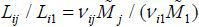 for all j . Therefore, we can express the occupational share in industry i ’s employment and industrial labor composite per capita as
From equations (5), (6), and (9), we have R / w = αi /[(1 – αi ) ki] . Accordingly, the ratio of capital stock per capita between two industries ( i and I ) satisfies
Also, from equations (4) and (5),
Combining this with equation (2), we have the following expression for the ratio of industrial employment.
At this point, I can compute the ratio of industrial employment and industrial capital per capita from equations (11) and (12) and hence industrial employment and capital stock. Substituting industrial employment and capital stock into equation (2), we can compute industrial output ( Yi ). Subsequently, we can compute the final output (Y ) from equation (1) and the industrial price ( pi ) from equation (4). The equilibrium level of rate of return ( R ) and the wage rate ( w ) are obtained correspondingly from equations (5) and (6). Lastly, substituting industrial employment into equation (9), we find the occupational employment in each industry (Lij ), from which occupational employment is determined, as follows:
Equations (9), (12), and (13) show how changes in exogenous productivity Ai and Mj affect industrial and/or occupational employment. For example, a rise in Ai would reduce the price of industry i , pi . When the elasticity of substitution across industries is less than one (ε <1 ), the amount of input in industry i would become smaller. The first bracket in equation (12) shows this substitution effect.
Each industry employs all occupations with different levels of intensity, meaning
that changes in occupational productivity (Mj ) also affect the industrial total factor productivity and hence industrial employment.
For example, a rise in Mj would increase Ṽi more in an industry that employs occupation j more intensively than others (i.e., an industry with a higher νij ). This would affect industrial employment through the second bracket on the right-hand
side of equation (12). More formally, industry i ’s production is 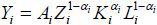 from equations (2) and (10), indicating that industry i ’s measured total factor productivity is
  , a combination of these values of Ai and Mj.
Similar to industrial employment, changes in both Ai and Mj affect occupational employment. Changes in Mj would alter occupational employment directly in equation (13) and indirectly through changes in industrial employment Li . Because changes in Ai alter industrial employment, they also affect occupational employment, as shown in equation (13).
Note that an increase in  would raise demand for occupation j (equation 13). Given that
  , an increase in is associated with an increase in Mj if σ >1 and a decrease in Mj if σ <1. Empirically, the literature finds elasticity of substitution across different
occupations to be less than one, implying that an increase in occupation-specific
productivity can be interpreted as technological progress substituting for labor in
occupation j .
, an increase in is associated with an increase in Mj if σ >1 and a decrease in Mj if σ <1. Empirically, the literature finds elasticity of substitution across different
occupations to be less than one, implying that an increase in occupation-specific
productivity can be interpreted as technological progress substituting for labor in
occupation j .
First, I define industry and occupation to connect the model with the data. The model’s industry and occupation are classified into thirteen industries and eight occupations referring to the Korean Standard Industry Classification (KSIC), Economic Activities in the National Account, and the Korean Standard Occupational Classification (KSOC) (see Table A1 for details). This classification yields 104 (= 13 industries × 8 occupations) industry-occupation pairs, but I report parameter values for three broad industries and three broad occupations in the main text for an intuitive explanation, while reporting detailed results in Appendix A. The three broad occupational groups are set as cognitive, routine, and manual occupations, following Acemoglu and Autor (2010), and the three broad industry categories are manufacturing, contact-intensive services, and other services. Classification of service industries is based on the industry’s employment-weighted average of work-from-home index, which I describe in detail later. Table 1 summarizes the industrial and occupational classifications.
The parameters of the final goods production function in equation (1) are the elasticity of substitution between industries (ε ) and the weight parameters ( γi ). From the equilibrium condition in equation (4), I formulate the following relationship:
I estimate the equation above by the iterated feasible generalized non-linear least squares (IFGNLS) method following Herrendorf, Rogers, and Valentinyi (2013). Because the substitution elasticity is greater than 0 and the weight parameters are located between 0 and 1, the estimation equation becomes
where the elasticity of substitution ( ε = 1 / (1 + eb )) and the weight parameters ( γi = eci / (1 + ∑eci)) are inferred from estimates of b and ci . The sample period is from 2005 to 2019, and the nominal and the real value added by economic activity from the National Accounts correspond to pi Yi and Yi , respectively.
The estimation results are shown in Table 2. The estimated value of the elasticity of substitution between industries is 0.503 within the range of the values in previous studies that report complementarities ( ε <1 ) in one-digit industry classification schemes.
The elasticity of substitution between occupations (σ ) governs how employment responds to a change in occupation-specific productivity (Mj ). Unfortunately, occupation-specific productivity (Mj ) and the elasticity of substitution between occupations (σ ) are not separately identified in our model. Therefore, I set the elasticity of substitution between occupations to 0.65, an average value of estimates in previous studies.1
Other parameters have been identified through the method of moments such that the data and endogenous variables of the model become similar in 2019. I calibrate the parameters to target the year 2019, not the average of 2010 to 2019, because one of the paper’s goals is to derive implications pertaining to structural changes over the medium run in the labor market after the pandemic. To do this, I assume that the year just before the pandemic represents the steady state and view the labor market after the pandemic as a transitional path from one steady state to another steady state. Note that this is somewhat different from the analysis of the business cycle, where average values over total sample periods are usually set as the steady state and where the analysis focuses on the short-run deviation from the steady state.
To be specific, I calibrate the values of νij such that they match the employment share by occupation and by industry, the value of αi to match the labor income share by industry, and the values of Ai,2019 to match the capital stock by industry as well as the level of aggregate output per total employment. Note that the model does not allow aggregate shocks to employment and the levels of total employment are given exogenously. That is, the model takes aggregate fluctuations as given and instead focuses on structural changes in the allocation of employment across industries and occupations. I therefore normalize the total number of workers in 2019 and the values of Mj,2019 to one. I then infer changes in the values of Ai , and Mj for the last decade (i.e., between 2010 and 2019) from the changes in employment by occupation and by industry. More specifically, I set the Ai,2010 to match industrial employment and the aggregate level of output in 2010 and the Mj,2010 to match occupational employment in 2010. I include detailed procedures for the calibration and data sources in Appendix A.
Table 3 summarizes the calibrated parameter values. The parameters for the occupational intensity levels (νij ) reflect each industry’s employment structure by occupation. For example, the manufacturing industry features the highest fraction of routine workers compared to the services industries. Similarly, I can also confirm that the share of manual occupations is largest in the contact-intensive services industry, implying that a shock to routine occupations would disproportionately affect the manufacturing industry more, and a shock to manual occupations would have a more severe effect on contact-intensive industries.
Not surprisingly, manufacturing is the most capital-intensive sector (the highest αi ). Among the service industries, the contact-intensive services sector is more labor-intensive than other services (αcontact < αother ).
Between 2010 and 2019, the sector-specific productivity of the contact-intensive services sector declined most rapidly among the three broad sectors, but this should not be interpreted as a decline in total factor productivity, a combination of the sector-specific productivity and occupation-specific productivity rates. The manufacturing sector experienced slower growth in sector-specific productivity than other services, possibly indicating that the rate of the decline of manufacturing employment slowed after the Great Recession. In addition, I could confirm that routine occupations experienced the fastest growth in their occupation-specific productivity rates in an occupational dimension.
The employment structure in the model is set to be equal to the data in 2019 in terms of construction. On the other hand, the model and the data do not match precisely in 2010 because only industrial shocks (Ai ) and occupational shocks (Mj ) are allowed to change between 2010 and 2019. Therefore, by examining how similar the employment structures in the model and data are in 2010, I check how well the model explains the employment structure in Korea before the pandemic.
Figure 1 compares the employment share of the model with data by industry and occupation in 2010. The x-axis is the share of employment by industry and occupation in the data, and the y-axis is the share of employment by industry and occupation in the model. The dotted line is the 45-degree line. As shown in the figure, the employment shares in the model are very similar to the employment shares by industry and occupation observed in the data with an R-square value of.987, indicating that the model is suitable for an analysis of the employment structure in Korea. Again, aggregate variables should precisely match the data through the calibration procedure by construction.
Note: The x-axis is the share of employment by industry and occupation in the data, and the y-axis is the share of employment by industry and occupation in the model. The dotted line is the 45-degree line.
Source: Author’s calculations.
In this section, I estimate industry- and occupation-specific shocks (Ai and Mj) from the employment dynamics during the COVID-19 periods, i.e., 2020 and 2021. Note that I refer to the industry- and occupation-specific shocks governing the employment dynamics during the COVID-19 periods as COVID-19 shocks. I then analyze the characteristics of COVID-19 shocks to understand the factors behind the employment dynamics during the pandemic.
The employment shocks during the COVID-19 period have a form that shows changes in Ai and Mj . I identify Ai and Mj that match employment in 2020 and 2021 as follows:
1) Set the total number of employed persons in 2020 and 2021 to the data.
2) Set arbitrary values for Mj ,t.
3) Set arbitrary values for AI ,t and kI ,t .
4) Find ki ,t based on kI ,t and equation (11).
5) Find Ai ,t for 2020 and 2021 from the following equation:
where  represents employment in industry i at time t in the data.
6) Iterate 3) to 5) over AI ,t and kI ,t until Kt is equal to the capital stock in 2019 and Y2020 / Y2019 (or Y2021 / Y2019 ) is equal to economic growth in the data.
7) Iterate 2) to 6) over Mj until , Lj,t / Lt in the model is equal to the data in 2020 and 2021.2
The procedure above produces Ai and Mj that match the thirteen industrial employment and eight occupational employment categories in 2020 and 2021 precisely. However, even if the thirteen employment by industry and eight employment by occupation categories coincide with the data, the detailed 104 (=13×8) employment cells by industry and occupation may not exactly coincide with the data. To check the accuracy, I compare the model with the data for the detailed 104 employment cells in Figure 2, finding that the model suitably explains the employment structure by industry and occupation during the pandemic. For example, the corresponding R-square outcomes between the occupational and industrial employment shares in the model and the data are 0.9975 and 0.9946 in 2020 and 2021, respectively.
Note: The x-axis is the share of employment by industry and occupation in the data, and the y-axis is the share of employment by industry and occupation in the model. The dotted line is the 45-degree line.
Source: Author’s calculations.
Although I identify the shocks that generate the employment dynamics during the pandemic, the economic meaning of these shocks is not straightforward. In the model, the only sources of exogenous variations are changes in Ai and Mj , which represent the productivity rates in each industry and each occupation. It would be natural to interpret these shocks as technological changes biased toward a certain industry or occupation when we focus on the long-run changes in the employment structure. However, there must be a much greater variety of shocks ongoing with regard to short-run fluctuations, such as markup, preference, and labor supply shocks, among others. Therefore, I would like to emphasize that the identified shocks herein should not be interpreted as structural sources of the variations in employment during the pandemic. Instead, the COVID-19 shocks identified herein should be understood as a combination of many structural shocks not explicitly reflected in the model.
However, the primary purpose of the identification of shocks is to gain an idea of which characteristics of an occupation or industry would be related to the observed changes in employment, rather than to delineate the contributions of various structural shocks on employment dynamics. For example, an occupation with higher infection risk would show lower employment caused by factors on both the demand and supply sides, and our exercise does not provide a clue as to exactly how much of the decrease in employment stems from a specific reason. Our exercise is still useful in that it defines the general nature of heterogeneity involved in the overall shocks to a certain occupation or industry, despite the fact that we do not know the contribution of each.
To provide economic implications with regard to COVID-19 shocks, I examine whether and how COVID-19 shocks are correlated with two variables that are suggested to be closely related to the pandemic in the literature: (1) the risk of infection and (2) easiness of remote work.
Recent studies utilize O*NET data to calculate the risk of infection index, and O*NET or the American Time Use Survey (ATUS) data to measure the ease of remote work (Adams-Prassl et al., 2020; Aum, et al., 2021c; Dingel and Neiman, 2020; Hicks et al., 2020; Mongey et al., 2021). O*NET asks experts and workers to give numerical answers to questions that capture detailed characteristics of an occupation, as defined by the Standard Occupation Classification (SOC) code. The ATUS data measure the amount of time people spend on various activities. In particular, it asks about “time worked from home,” which varies across industries as well as occupations.
I adopt the infection risk index and index for ease of remote work from Aum, Lee, and Shin (2021b) (henceforth work-from-home or wfh index) by industry and by occupation. The infection risk index is obtained using O*NET data examining the characteristics of each occupation in the US. Specifically, in O*NET, the degree of physical contact and exposure to diseases and infections are investigated and scored for each job. The infection risk index is the average value of two – the degree of physical contact and exposure to diseases and infections – after the standardization of each score. The work-from-home index is calculated using the weighted average of actual working at home in ATUS by industry and occupation. Finally, to match the indexes with our COVID-19 shocks, I assign US Census occupation codes and NAICS (North American Industry Classification System) to one-digit KSOC and KSIC.
Figure 3 shows the infection risk index against the work-from-home index by industry and occupation in Korea. Specifically, the x-axis is the work-from-home index (wfh) and the y-axis is the infection risk index (infect). The size of the circle represents the share of employment by industry and occupation in 2019. There is a negative (-) correlation between the two indexes, meaning that jobs with a lower risk of infection are generally more easily done at home. However, there is also considerable deviation from the regression line, implying that one index cannot completely represent the other and that the two indexes need to be examined separately. Aum, Lee, and Shin (2021b) also emphasized that the relationship between two indexes is far from tight, with an R-squared value only 0.034.
Note: The x-axis is work-from-home index (wfh), and the y-axis is the infection risk index (infect). The size of the circle represents the share of employment by industry and occupation in 2019.
Source: Author’s calculations based on O*NET, ATUS, and EAPS.
I estimate the following regression to examine the relationship between COVID-19 shocks and the two indexes using employment by industry and occupation as a weight.
where wfh is the work-from-home index (by industry and by occupation), infect is the risk of infection index (by occupation), Mj,t is an occupation-specific shock, and Ai,t is an industry-specific shock. Note that β1 > 0 if jobs with lower wfh outcomes (i.e., more difficult to do remote work) were hit harder by adverse employment shocks, and β2 < 0 if jobs with higher infection risk were hit harder by adverse employment shocks. The regression analysis would guide us to a better understanding of the underlying sources of the variation in employment shocks by industry and occupation during the pandemic.
Table 4 shows the estimation results, which deliver three main results. First, in both 2020
and 2021, we have  and
and  , confirming the intuition that jobs that are more difficult to do remotely and with
a higher risk of infection were hit harder both by occupation shocks and industry
shocks, although these relationships were not always significant.
, confirming the intuition that jobs that are more difficult to do remotely and with
a higher risk of infection were hit harder both by occupation shocks and industry
shocks, although these relationships were not always significant.
Note: Standard error in parenthesis. *, **, and ** indicate significance at the 90%, 95%, and 99% percentiles, respectively.
Source: Author’s calculations.
Second, the relationships vary over time. In 2020, when employment rapidly declined, COVID-19 shocks show a significant correlation only with infection risk. However, the work-from-home index began to show a significant correlation with COVID-19 shocks in 2021, as employment began gradually to recover. On the other hand, the coefficient of infection risk ( β2 ) becomes smaller in 2021 compared to this value in 2020.
Third, both indexes, risk of infection and work-from-home, have tighter relationships with COVID-19 shocks in an occupational dimension than in an industrial dimension. For example, the R-squared outcome in the regression with occupational shocks is 0.300, whereas that with industrial shocks is only 0.070. In addition, the t-value corresponding to the relationship between the work-from-home index and industrial shocks was 1.69, significantly smaller than with occupational shocks, at 7.28. This is not surprising given that the easiness of remote work is mainly related to the tasks a worker performs as opposed to the industry in which she/he works. I interpret this as meaning that occupational heterogeneity plays a more critical role in deriving the employment structure during the pandemic.
As of January of 2022, the COVID-19 virus continues to spread with multiple variants, and it remains uncertain as to when the pandemic will end and how COVID-19 will affect the employment structure in the future. Nevertheless, I attempt to derive implications related to the post-pandemic employment structure in view of our model.
The results in Section 4 suggest that COVID-19 raised the cost of employing contact-intensive tasks (specifically jobs for which the work-from-home is more difficult). According to the literature on directed technological change (e.g., Acemoglu and Restrepo, 2018, among others), an increase in the cost of employing contact-intensive tasks provides incentives to implement technological changes to replace these tasks. A natural question is whether such technological changes are feasible.
Although the literature has actively investigated the impact of technological changes on the labor market structure, it did not pay much attention to how contact-intensive each job is and whether new technology can replace contact-intensive tasks. However, even before the pandemic, recent technological changes enabled the replacement of contact-intensive tasks to some extent. For example, the widespread use of food-delivery applications through various platforms has replaced food-serving services in the restaurants with fewer workers. Many other examples indicate similar possibilities, such as the expansion of telemedicine due to the CPRSA Act in the US, the provision of online education services through the development of MOOC, or the development of smart-finance applications. Reflecting such trends, the Ministry of Science and ICT (2020; 2021) reports that the amount of O2O (online-to-offline) transactions in Korea grew by 22.3% in 2019, even before the pandemic, and its growth rate accelerated to 29.6% in 2020 through the pandemic. Therefore, I consider the acceleration of technological changes to replace contact-intensive tasks as a scenario that merits investigation.
The baseline scenario is that only past trends continue for five years, with no additional effects from COVID-19 appearing. I label this scenario as the baseline scenario, or Scenario 1.
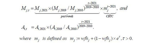
Scenario 1. (past trends) For 2022 ≤ t ≤ 2026, occupation- and industry-specific productivity evolve as follows:
The expression above may seem complicated, but it merely says that the sector-specific and occupation-specific productivity rates grow at the average rate of growth between 2010 and 2019.
Compared to this scenario, I consider an alternative scenario in which the replacement of contact-intensive tasks will accelerate due to technological change biased toward contact-intensive task (CBTC) in the coming years. To reflect such technological changes, I assume that occupations with a lower work-from-home share will experience a more rapid increase in occupation-specific productivity compared to earlier trends. Hence, when new technologies replace contact-intensive tasks, occupations having more contact-intensive tasks will become relatively more productive. As shown in equation (13) in Section 2, a faster increase in an occupation’s productivity reduces its demand when occupations are complementary to each other (σ <1). Intuitively, firms allocate fewer resources to more productive tasks when tasks are complementary to each other.
To be specific, the alternative scenario (scenario 2) is expressed as follows:
Scenario 2. (past trends + COVID-19) For 2022 ≤ t ≤ 2026 , occupation- and industry-specific productivity evolve as follows:
Note that Scenario 2 is identical to Scenario 1 except for the mj in the first equation. The additional term mj captures CBTC, implying that the productivity rates of occupations that are difficult to do from home increase more rapidly. In other words, owing to CBTC (mj ), Mj > Ml when 1 – wfhj > 1 – wfhl . Note again that the demand for occupation j falls when Mj becomes higher when σ <1 (equation 13).
The parameter τ governs the speed of CBTC and determines the distance between the productivity of the highest wfhj and the productivity of the lowest wfhj . I set τ = 0.14 , referring to the average speed of divergence between the highest Mj and the lowest Mj between 2010 and 2019, the pre-pandemic period.
Contrary to the previous section, the simulation exercise in this section is structural because I simulate a situation in which technological change is biased toward contact-intensive tasks. In other words, the simulation seeks to determine the structural effect of contact-intensive-task-biased technological changes on occupational and industrial employment rather than accurately to predict the employment dynamics after the pandemic. In this sense, I would like to clarify that the previous exercise does not provide evidence but suggests the possibility of CBTC. This is certainly a limitation of this analysis. Finding evidence of CBTC would require more data and analyses after the pandemic. This can be examined in future research.
I simulate the model and the obtained equilibrium employment structures ( Li,j,t / Lt ) under Scenario 1 and Scenario 2. Figure 5 depicts the occupational structures under the two scenarios. The line demarcated by the circle shows the observed employment share between 2005 and 2020. Not surprisingly, there was a declining trend in the routine employment share (-2.5%p between 2010 and 2021). Accompanying this trend, the cognitive employment share and manual employment share rose by +0.3%p and +2.3%p, respectively.
Note: The line marked with circles is the observed employment share in the data; the black dotted line is Scenario 1, and the gray solid line is Scenario 2.
Source: Author’s calculations.
Similar to the continuous decline of routine employment before the pandemic, the routine employment share continues to fall by as much as -1.7%p for the next five years under the baseline scenario (solid gray line). At the same time, the cognitive employment share rises by +1.1%p, and the manual employment share rises by +0.6%p, a continuation of job polarization (or the declining trend of routine employment).
When the replacement of contact-intensive task accelerates (black dotted line, Scenario 2), however, the manual employment share changes, turning negative (+0.6%p → -0.3%p). A reduction in the demand for manual employment translates into greater demand for routine and cognitive employment than in previous trends, leading to a smaller decline of the routine employment share (from -1.7%p in Scenario 2 to -1.1%p in Scenario 2) and even higher increases in the cognitive employment share (from +1.1%p in Scenario 1 to +1.4%p in Scenario 2).
Equation (13) provides an idea as to why the replacement of contact-intensive tasks
reduces the demand for manual workers. Because σ <1 in our calibrated model, an increase in Mj translates into a fall of  , which leads to a reduction in Lj in Equation (13). Because mj is higher for manual workers than for other occupations, manual workers experience
lower demand compared to other types of employment. In other words, manual workers
tend to have tasks that are difficult to complete from home (relatively lower wfhj ) and hence are substituted more by technological changes that replace tasks that
cannot be done at home.
, which leads to a reduction in Lj in Equation (13). Because mj is higher for manual workers than for other occupations, manual workers experience
lower demand compared to other types of employment. In other words, manual workers
tend to have tasks that are difficult to complete from home (relatively lower wfhj ) and hence are substituted more by technological changes that replace tasks that
cannot be done at home.
I now turn to the industrial structure. Figure 6 shows the industrial employment structure under the two scenarios. In the data, the manufacturing employment share fell (-1.5%p from 2010 to 2021) and services employment increased through the process of structural transformation (circle-demarcated line). Within the service industry, the increase of line employment share focused on contact-intensive services (+2.6%p), whereas the share of other services (mostly high-skilled) experienced a decline (-1.1%p).
Note: The line marked with circles is the observed employment share in data; the black dotted line is Scenario 1, and the gray solid line is Scenario 2.
Source: Author’s calculations.
When the previous trend continues (Scenario 1), the manufacturing employment share decreases by -1.0%p over the next five years, while the employment share of contact-intensive services increases by +1.5%p and the employment share of other services falls by -0.5%p. However, as the replacement of contact-intensive tasks accelerates after the pandemic (Scenario 2), the demand for contact-intensive services will be reduced by -0.3%p over the next five years a -1.8%p reduction from +1.5%p in Scenario 1. As the demand for contact-intensive services decreases, the decline in manufacturing will ease, shifting from -1.0%p in Scenario 1 to -0.003%p in Scenario 2. Also, the demand for other services will boost the employment share of these workers by +0.3%p.
The simulation results demonstrate that the acceleration of contact-intensive replacement technological changes (or CBTC) would alleviate the structural changes in employment observed in the past, such as job polarization. This would occur because jobs with more significant portions of contact tasks (i.e., remote work being more difficult) are different from jobs that involve routine tasks, which have been replaced heavily by earlier technological changes, also known as the IT revolution.
It is important to note that these results should not be interpreted as meaning that routine tasks will not be replaced in the future. Instead, they suggest that a broader range of jobs, both routine tasks and contact-related tasks, may be in danger after the pandemic given the more recent technological changes that have occurred. I highlight the potential acceleration of the former type of automation due to the pandemic and present related implications with regard to occupational or industrial employment structures.
The CBTC scenario (Scenario 2) includes technological changes reflecting past trends as well as the acceleration of contact-intensive task replacement. Although a contact-intensive task is different from a routine task, they are not mutually exclusive. In other words, jobs intensive in routine tasks may or may not be intensive in contact tasks. For a more precise interpretation, I classify jobs by both routineness and contact-intensiveness in Table 5. I classify jobs with a work-from-home index below average as contact-intensive jobs and those with a work-from-home index above average as non-contact-intensive jobs. This classification of routine and non-routine jobs follows the literature, e.g., Acemoglu and Autor (2010).
Note: 1) Contact-intensive jobs are those for which the wfh index is below average, and non-contact-intensive jobs are those for which the wfh index is above average, 2) The classification of routine and non-routine jobs follows Acemoglu and Autor (2010).
Before the pandemic, a widely accepted view with regard to the labor market structure was that routine jobs had disappeared, regardless of their degree of contact-intensiveness. Our simulation is based on the possibility that contact-intensiveness can serve as an additional dimension of future technological changes due to the COVID-19 pandemic. Therefore, among routine jobs, the share of routine and contact-intensive jobs will decrease further, adding to the previous decline. In addition, the share of non-routine and non-contact-intensive jobs will increase more rapidly than in the past. Most interesting is that the demand for non-routine and contact-intensive jobs, i.e., manual jobs, shifts from increasing to decreasing with the widest gap between the two scenarios, as highlighted in Section 5.C.
Table 6 compares the employment composition of manual, routine, and cognitive jobs in 2020 in Korea. Manual jobs have a higher proportion of temporary and daily workers than other jobs (45% vs. 15% or 10%), and the share of low-educated (up to high school) workers is also higher than in the other cases (78% vs. 56% or 13%). Meanwhile, more elderly people (over age 60) work manual jobs than in other cases (31% vs. 18% or 6%), meaning means that the reduced demand for manual workers due to the pandemic will burden mostly socio-economically vulnerable workers, which calls for policies supporting vulnerable groups in the labor market.
I study how COVID-19 affected the labor market through the lens of a general equilibrium model with multiple industries and occupations. I calibrate the model with Korean data and identify industrial and occupational COVID-19 shocks that derive employment dynamics in 2020 and 2021, when COVID-19 hit the Korean labor market.
I find that COVID-19 shocks correlate significantly with both infection risk and ease of work-from-home by occupation and industry. As the pandemic progressed, however, the correlation with infection risk weakened, whereas the correlation with the easiness of work-from-home strengthened. Moreover, the relationship is more robust in the occupational dimension than in the industrial dimension.
Based on this finding, I investigate how much, and in which direction, labor market structure would be affected if future technological changes accelerated the replacement of contact-intensive tasks (i.e., tasks that cannot be done at home). The simulation results show that the upward trend in manual workers’ employment share will shift to a declining trend due to the pandemic. This result stands in contrast with the earlier trend of job polarization in which only routine workers showed a declining employment share. The analysis suggests that whether or not a job requires contact-intensiveness can play an essential role in shaping the future labor market structure; moreover, if it occurs, such a change calls for policies that support socio-economically vulnerable groups, distributed mainly in manual jobs.
1. Classifications of Industry and Occupation
The classification of industries is mainly based on the classification of national accounts by economic activity; it is subsequently linked to the KSIC. I exclude agriculture, forestry and fishing and the public. Occupational classification is based on the KSOC, and I also exclude skilled workers in agriculture, forestry and fisheries, as in these cases it is difficult to connect with the data on infection risk and the work-from-home index later. Table A1 compares the classification in the model and the data.
2. Estimation of production function parameters
From the equilibrium condition in equation (4), we have the following relationship:
I estimate the above equation by the iterated feasible generalized non-linear least squares (IFGNLS) method following Herrendorf, Rogers, and Valentinyi (2013). The sample period is from 2005 to 2019, and the nominal and the real value added by economic activity from the National Accounts correspond to pi Yi and Yi , respectively. The estimation results are in Table A2.
Note: Standard errors in parenthesis.
Source: Author’s calculations.
3. Calibration
The elasticity of substitution between occupations (σ ) governs how employment responds to a change in occupation-specific productivity (Mj). I set the elasticity of substitution between occupations to 0.65, an average value of estimates in previous studies (Aum, Lee, and Shin, 2018; Aum, 2020; Lee and Shin, 2017; Duernecker and Herrendorf, 2020).
Other parameters have been identified through the method of moments so that the data and endogenous variables of the model are similar in 2019. I calibrate the values of νij to match employment by industry and by occupation; in all cases αi matches labor income shares by industry and i A matches capital stock by industry as well as the aggregate level of output, in the year 2019. Because the model does not have aggregate shocks to generate aggregate fluctuations, it takes any variations in the aggregate variable exogenously. Therefore, I normalize total employment in the year 2019 to one.
To be specific, the detailed procedure for the calibration is as follows.
1) Normalize Mj,2019= 1 for all j .
2) Set an arbitrary value of AI ,2019 .
3) Find νij from equation (9), Mj,2019= 1 , and employment by occupation and industry in 2019; that is,νij = Lij,2019 / Lj,2019 .
4) From equation (10), we have  .
.
5) Determine αI from 1 – labor shareI,2019 in the data. Then, αi = 1 / [1+(1 – αI) kI,2019 / (αIki,2019)] from equation (11).
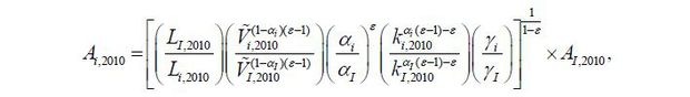
6) The industry-specific productivity Ai,2019 is then
from equation (12).
7) Iterate over AI ,2019 until the aggregate output in the model is equal to the data.
In our model, the time-varying exogenous variables are occupation-specific productivity Mj and industry-specific productivity Ai as well as aggregate variables. To have changes in the values of Mj and Ai corresponding to structural changes in the labor market before the pandemic, we identify the best matches of Mj,2010 and Ai,2010 to the observed changes in employment by industry and occupation between 2010 and 2019.
Specifically, from equation (9),
for all i∈(1,⋯, I ) . Denoting  , establish the occupation specific productivity in 2010 via
with M8,2010 = 1 .
Lastly, the Ai,2010 values are obtained using the equation
where AI ,2010 is set to match the aggregate output in the model and that in the data in 2010.
Given the calibrated values of αi , we can compute the value of the rate of return on capital ( R ) in the model. The rate of return on capital implies that β = 0.987 , with a depreciation rate (δ ) of 0.05, which is the consumption of fixed capital divided by the net capital stock in 2019 in the Korean National Accounts.
Table A3 summarizes the calibrated parameter values.
4. Data Construction
The data for the output, capital, and labor income shares are obtained from the value added by economic activity (Tables 10.2.1.3, 10.2.1.4), the net capital stock (Tables 14.7.1, 14.7.2), employee compensation (Table 10.3.1.2) by industry, and the operational surplus of households (Table 10.4.2) in the Economic Statistics System (ECOS) of the Bank of Korea. In particular, I compute the labor income shares by industry from the compensation of employees divided by value added net of operational surplus of households by industry. Because the Bank of Korea provides data on the operational surplus of households at the aggregate level only, I distribute this data to each industry based on the share of self-employed in each industry.
The data for employment come from the Economically Active Population Survey (EAPS) from MDIS (Microdata Integrated Service). Employment by industry and occupation were based on the average number of employed persons from March to August of 2019 in the Economically Active Population Survey (EAPS). I restrict employment data from March to August because the COVID-19 shock started in March of 2020 and the microdata from the 2021 EAPS were available only until August at the time of the analysis. Therefore, employment in 2010, 2019, 2020, and 2021 in the model correspond to the average number of employed persons from March to August of 2010, 2019, 2020, and 2021, respectively.
Finally, the aggregate level of output comes from the Gross Domestic Product, Table 10.2.2.4, in ECOS.
This paper is revised version of Aum, 2021 (forthcoming), “Post-COVID19 Labor Market Structure,” in Kyu-Chul Jung (ed.), Chapter 3, Macroeconomic Challenges and Policy Direction for the Post-COVID Era, KDI (in Korean).
The elasticity of substitution between occupations ranges from 0.56 to 0.81 in previous studies. Specifically, Aum, Lee, and Shin (2018) find a value of 0.81, Aum (2020) finds 0.58, Lee and Shin (2017) show a value of 0.70, and Duernecker and Herrendorf (2020) report 0.56.
, & (2018). The Race between Man and Machine: Implications of Technology for Growth, Factor Shares and Employment. American Economic Review, 108(6), 1488-1542, https://doi.org/10.1257/aer.20160696.
, , & . (2018). Computerizing Industries and Routinizing Jobs: Explaining Trends in Aggregate Productivity. Journal of Monetary Economics, 97, 1-21, https://doi.org/10.1016/j.jmoneco.2018.05.010.
, & (2013). The Growth of Low-skill Service Jobs and the Polarization of the US Labor Market. American Economic Review, 103(5), 1553-1597, https://doi.org/10.1257/aer.103.5.1553.
, , & (2003). The Skill Content of Recent Technological Change: An Empirical Exploration. The Quarterly Journal of Economics, 118(4), 1279-1333, https://doi.org/10.1162/003355303322552801.
, , & (2013). Two Perspectives on Preferences and Structural Transformation. American Economic Review, 103(7), 2752-2789, https://doi.org/10.1257/aer.103.7.2752.