- P-ISSN 2586-2995
- E-ISSN 2586-4130

This study examines the impact of sentiment shock, which is defined as a stochastic innovation to the Housing Market Confidence Index (HMCI) that is orthogonal to past housing price changes, on aggregate housing price changes and housing price volatility. This paper documents empirical evidence that sentiment shock has a statistically significant relationship with Korea’s aggregate housing price changes. Specifically, the key findings show that an increase in sentiment shock predicts a rise in the aggregate housing price and a drop in its volatility at the national level. For the Seoul Metropolitan Region (SMR), this study also suggests that sentiment shock is positively associated with one-month-ahead aggregate housing price changes, whereas an increase in sentiment volatility tends to increase housing price volatility as well. In addition, the out-of-sample forecasting exercises conducted here reveal that the prediction model endowed with sentiment shock and sentiment volatility outperforms other competing prediction models.
Sentiment, Housing Price, Out-of-sample Forecasts, Seemingly Unrelated Regression
G12, R30
“Housing has also been a source of endless fascination for the general public, because we live in houses, we work on them every day, and our sense of our individual social position is tied to the kind of house we live in.” - Shiller (2005)
The objective of this study is to quantify the impact of housing-market-related sentiment shock on housing price changes and housing price volatility in the short run. In addition, this paper examines the role of sentiment shock volatility in the determination of future housing price changes and housing price volatility.
To estimate sentiment shock and how it affects the housing market in Korea, the Housing Market Confidence Index (HMCI), which represents the current assessment of the housing market, is utilized. The empirical relationships between sentiment-related variables and housing price-related variables are investigated under an appropriate empirical framework. Specifically, we deploy a simultaneous regression approach (e.g., seemingly unrelated regression) in which the dependent variables are housing price changes and housing price volatility. We design the empirical model specifications such that sentiment shock and sentiment shock volatility serve as key explanatory variables in the model, which is based on the theoretical setup introduced in Section III. In addition, we investigate whether the estimated sentiment shock can serve as a good predictor of the evolution of future housing prices in out-of-sample forecasting exercises
Sentiment, which can be defined in various ways and is frequently used as a synonym for the psychology of market participants, is considered one of the major driving forces in numerous economic activities and markets, as claimed by Keynes (1936). While the semantic aspect of the word ‘sentiment’ has the connotation of various cognitive biases to which humans are exposed, we construct the sentiment shock variable such that it captures not only sentiment components in the HMCI but also unobserved information about housing market fundamentals, which may not be reflected housing prices at the time of collection. From this standpoint, the discussion of sentiment shock and its role in the determination of asset prices is closely related to the debate on market efficiency (i.e., the efficient market hypothesis).
Sentiment or psychology in the residential real estate market can play a crucial role in shaping the dynamics of the housing market because, in the residential real estate market, unlike financial markets such as the stock market, the tools (e.g., short selling) for adjusting housing prices are relatively limited with regard to their use, even if housing prices deviate from the fundamentals. Given that households often fail to make rational choices due to various psychological biases, the residential real estate market operating with anticipation of the future may undergo drastic changes due to extreme optimism or pessimism. The importance of the residential real estate market in Korea is also becoming paramount in the sense that residential real estate accounts for the largest portion of household assets. Most importantly, most residential property purchases are partially financed by mortgage loans from Korean banks, suggesting that the stability of the banking system of Korea largely depends on the conditions of the housing market.
Consistent with the related literature, this paper documents the importance of sentiment in Korea’s housing market, demonstrating that there is a close association between sentiment shock and future housing prices. In addition, the study also reveals that not only the sentiment shock level but also the magnitude of its variability are important determinants of future housing prices in the short run, as predicted by the simple theoretical setup introduced in Section III. While related works primarily focus on the sentiment level itself, the aspect of sentiment volatility is comparatively neglected. In this regard, this study contributes to the literature by filling this gap, incorporating the sentiment volatility into the formal analysis.
In addition, the paper also demonstrates that a simple forecasting model with a sentiment shock variable and sentiment volatility yields better forecasting accuracy than benchmark forecasting models (e.g., AR(p) models).
The contributions of this study can be summarized as follows. First, the roles of sentiment shock in the Korean housing market and its significance have rarely been tested. More importantly, this study explicitly considers sentiment volatility as one of the key drivers of housing price dynamics. Second, the study attempts to reveal not only the link between sentiment shock and the housing price level but also the link between sentiment shock and housing price volatility, an aspect which is not been examined in thus far in the literature. Third, this paper is the first study to verify the forecasting power of sentiment shock for future housing prices in the short run.
This paper is structured in the following format. In the following section, we review a few closely related studies that mainly focus on empirical validations of the importance of sentiment shock in the housing market. In Section III, we introduce a simple theoretical model for the determination of the stochastic process of housing price changes in the presence of sentiment shock. In Section IV, we introduce the empirical framework in which the paper’s primary objectives are properly fulfilled. In Section V, we provide a brief description of the data used for empirical analysis. In Section VI, we report key results of the estimation and discuss them. In Section VII, the paper concludes with remarks.
Recognizing the increasing importance of sentiment in the determination of asset prices, previous studies in this area attempt to quantify sentiment in a specific market in various ways. In relation to stock markets, the seminal paper by Baker and Wurgler (2006) uses mutual fund flows, dividend premia, and closed-end fund discounts as proxies for sentiment to construct a sentiment index for the stock market. They show that the sentiment index can explain a large proportion of the cross-sectional variation in stock returns. This line of works, which emphasizes sentiment as a key source of the determination of asset prices, also includes Edmans et al. (2007), Baker et al. (2012), Tetlock (2007), Tetlock et al. (2008), and Pyo and Kim (2021).
With regard to the housing market, most studies focus on measuring the housing market sentiment level from text-based sources. For example, Soo (2018) quantifies the level of sentiment for 34 cities in the U.S. and examines its impact on future housing prices using the tone of local newspaper articles with the help of a textual analysis. This novel approach based on text attempts to quantify emotional contents in various text sources available to grasp the state of the collective psychology of market participants, rather than resorting to a survey-based sentiment index such as the University of Michigan’s Survey of Consumers or the index in Case and Shiller (2003).
Other text-based studies aiming to estimate housing market sentiment and study its impact on housing prices include Beracha et al. (2019), Hausler et al. (2018), and Walker (2014), all of which provide supporting evidence of the economic significance of sentiment for housing prices. For example, Beracha et al. (2019) quantify1 the level of optimism/pessimism in the housing market in the U.S. using 35,000 real-estate-related articles in the Wall Street Journal. Their findings suggest that there are intertemporal links between sentiment and the returns on commercial real estate properties, showing that sentiment as reflected in news media can help predict future returns on commercial real estate. Similarly, Hausler et al. (2018) apply a machine-learning algorithm (e.g., support vector machine) to measure the news-based sentiment level of the U.S. housing market and examine its statistical relationship with future returns in the commercial real estate under the VAR framework. In line with related studies, their study shows that there is a positive relationship between the lagged sentiment indicator and returns on commercial real estate. Walker (2014) uses a similar approach in the U.K. housing market, showing that news-based sentiment affected housing prices in the U.K. through a Granger-causality mechanism during the housing boom period (1993-2008), but not during other periods. This evidence suggests that the news media have influenced the views of market participants in the housing market.
While this text-based approach has several advantages over the conventional method,2 in this paper we use a survey-based housing market confidence index as a benchmark upon which the sentiment shock variable is devised. This is done for the following reasons. First, the housing market confidence index is published monthly and thus timely assessments of the current housing market conditions are not substantially limited. Second and more importantly, the construction of the housing market sentiment variable from text data inherently involves a researcher’s ad-hoc assumptions which regard to which positive/negative words to choose when computing the relative strength of the two types of sentiment (i.e., positive versus negative).
On the other hand, the literature also reports that sentiment in other asset markets can indeed have an impact on housing market performance outcomes. For example, Zheng and Osmer (2021) show that housing price returns tend to be higher when pessimistic sentiment prevails in the U.S. stock market. One interesting feature of the pattern of housing prices is the asymmetry in its responses to sentiment variations with regard to the stock market; it is found that housing prices are more sensitive to negative sentiment in the stock market than to positive sentiment.
Studies of housing market sentiment are not limited to text-based approaches. For example, Stefani (2021) shows that the leveraged investment behavior of households regarding their housing purchases is closely associated with the sentiment inferred from the University of Michigan’s Survey of Consumers. Specifically, the study documents that an increase in the sentiment index tends to lead to a higher leverage ratio of long-term fixed-rate mortgage loans. Though this study does not directly deal with housing prices, it demonstrates that household sentiment is an important element of housing purchase decisions. Zheng et al. (2016) also examine the impact of the survey-based consumer confidence index on housing prices in China’s urban cities. Though they found that innovations in the survey-based confidence index predict housing price appreciation and an increased volume of transactions, the magnitude of the strength of the relationship varies depending on other characteristics of a city, such as demographic factors and the elasticity of the housing supply.
In this section, we develop a simple theoretical model to show the equilibrium returns on residential properties and equilibrium volatility are functions of household sentiment shock and the volatility of sentiment shock. In addition, this model provides the theoretical justification for using a seemingly unrelated regression model as defined in the following sections on the empirical model specification.
The model we are proposing here is a modified version of the concepts in Danielsson et al. (2010), though here we introduce a sentiment element into household expectations of future housing price changes. In the model, this stochastic sentiment acts as a unique seed of uncertainty to drive the evolution of equilibrium housing price changes and the corresponding volatility, and time is continuous.
We consider a representative household endowed with capital ( Kt ) and we assume that house purchases are partially financed by mortgage loans ( Bt ). The budget constraint our hypothetical household is given by Eq. (1):
where Pt is the market price of a house and θt denotes the demand for houses. Assuming continuous time, the capital gains ( dKt ) from purchasing housing properties can be written as Eq. (2):
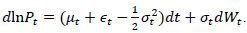
Let us also assume that the equilibrium housing price diffusion shows geometric Brownian motion, as depicted in Eq. (3):
where μt is the rate of housing price changes, σt denotes the volatility of housing price changes, and Wt follows a standard Wiener process.
The household is assumed to have a stochastic sentiment shock ( εt ) of the subjective perception of the true return of housing prices ( μt ), such that
where dεt = σεdWt. Note that σε captures the volatility of the household’s sentiment, which we label as ‘sentiment volatility’ and sentiment shock ( εt ) is orthogonal to the true return on housing prices ( μt ).
Conditional on the subjective belief ( xt ), the expected capital gain from the investment in housing properties is given by Eq. (5):
Given the equilibrium volatility of housing price changes, the variance of the capital gain is expressed by Eq. (6):
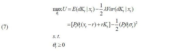
In this model, assuming that the household is risk-averse, the household seeks to maximize their mean-variance utility over the capital gains from their investment in housing properties:
where λ is the coefficient of risk aversion. Note that short-selling of housing properties is not allowed in this setup ( θt ≥ 0 ) given that tools for implementing short-selling strategies on housing properties are very limited in the Korean housing market.
The first-order condition for optimality of the mean-variance utility maximization problem above yields the following demand function for housing properties:
Assuming a fixed supply of housing properties ( θ ) in the short run, the equilibrium price of a house can be expressed as:
Note, from Eq. (9) that we can infer
Applying Ito’s lemma to the first term in Eq. (10), we have
where  and
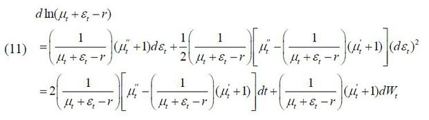
and  In a similar fashion, the diffusion process of the second term in Eq. (10) can be
obtained by applying Ito’s lemma as shown in Eq. (12):
In a similar fashion, the diffusion process of the second term in Eq. (10) can be
obtained by applying Ito’s lemma as shown in Eq. (12):
where  and
and 
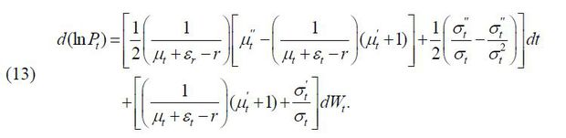
Substituting the terms in Eq. (10) with those in Eq. (11) and Eq. (12), we have
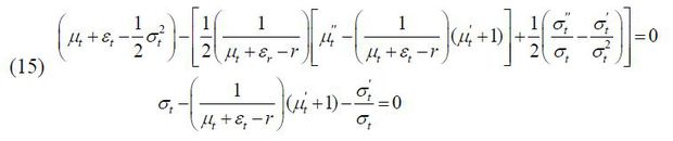
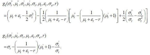
The rational expectation equilibrium (REE) can be obtained by comparing the perceived return and the perceived volatility to the realized return and the realized volatility. Hence, the equilibrium return and the equilibrium volatility can be expressed as a set of equations meeting the following conditions:3
Rearranging Eq. (14) yields
Eq. (15) implies that the REE return and volatility can be represented by a system of nonlinear differential equations such that
where
Eq. (16) is indeed a system of nonlinear differential equations with no closed-form solutions. However, we can at least roughly infer that the solution of endogenous variables (i.e., housing price changes and corresponding volatility) in the above system are functions of exogenous variables in the model (i.e., sentiment shock, sentiment volatility, interest rate), as shown in Eq. (17).
Because no closed-form solutions to the system of nonlinear differential equations in Eq. (16) exist, in the following section we resort to several empirical models to examine the impact of sentiment shock on housing prices and volatility. This approach approximates a comparative static analysis of the theoretical model.
In this section, we describe the empirical framework in which key research questions are addressed.
Given that the key objective of this study is to quantify the effects of variations of household sentiment, which is weakly correlated with the fundamentals of the housing market, it is imperative initially to define and estimate the level of sentiment poised by market participants in the housing market.
This study derives the sentiment shock related to the housing market by utilizing the Housing Market Confidence Index (HMCI). The HMCI published by the Korea Research Institute for Human Settlements (KRIHS), regarded as the most reliable housing-market confidence index, is the only quantitative indicator of the housing market in Korea.
The HMCI is constructed from a monthly survey of households and real estate brokers. The questionnaire includes several questions. For example, in the case of households, it contains the residential housing price level compared to the previous quarter, the neighboring housing price level compared to the previous quarter, the time to buy housing, and the time to sell housing. The surveys for real estate brokers contain questions about the level of housing transaction intensity in their business areas, selling/buying pressure levels, and the level of housing prices in their business areas compared to the previous month.
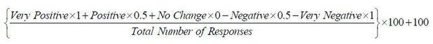
The HMCI is designed such that it is calculated first for each question, after which the sub-indexes for each question are combined to create the final index. The questions are multiple-choice types (e.g., very positive, positive, no change, negative, very negative) for market conditions (e.g., price, transactions), and scores are calculated by multiplying the number of responses by a weighting factor. The exact formula for calculating the final index is given below.
Note that with this construction, the HMCI ranges from 0 to 200. A score exceeding 100 indicates that there are more respondents who reported that prices or transactions have increased compared to previous periods. The HMCI is usually categorized into three phases: (a) if it is less than 95, this indicates a downward phase; (b) if it is 115 or more, it can be seen as an upward phase; and (c) it is classified as a steady phase if it is between 95 and 115.
Figure 1 depicts the evolutionary trends of the HMCI at the Seoul Metropolitan Region (SMR) level and at the national level along with housing price changes. This figure demonstrates that most periods can be classified above the steady phase for the last decade, except the first two months of 2019. The sharp deterioration of the HMCI at the beginning of 2019 does not appear to have reversed the rising trend of housing prices in Korea.
Note: The solid line denotes the housing price change computed from the housing price index compiled by KB Real Estate. The dotted line denotes the Housing Market Confidence Index published by the KRIHS.
In this study, housing market sentiment shock (HMSS), which is distinct from the HMCI but closely related to it, is defined through two major steps. In the first step, we estimate the following regression equation using the HMCI and the past housing price changes.
In this equation, et ~ N(0, σ2) , HMCI denotes the housing market confidence index, and HPC stands for housing price changes.4
In the second step, we define sentiment shock as the residual of the HMCI not explained by previous housing price changes,
where HMSS stands for housing market sentiment shock.
Note that the HMCI accounts for the prospects of respondents with regard to the future status of the housing market, as well as other market information. If housing prices are determined by both types of information closely related to the fundamentals of the housing market and the sentiment of market participants, the HMSS defined above can then be interpreted as a variable that captures both unobserved fundamental information and unobserved sentimental components in households’ prospects concerning the housing market.
The degree of the relative importance of sentiment with regard to the sentiment shock variable may depend on the efficiency of the housing market; if the housing market is very efficient, in the sense that prices quickly incorporate information regarding housing market fundamentals, much of the sentiment shock will be governed by non-fundamental elements. Otherwise, sentiment shock may capture both the sentimental component and unobserved housing market fundamentals.
The sentiment shock values estimated from Eq. (19) are plotted in Figure 2. Although the two sentiment shock variables at the SMR level and the national level do not move together perfectly, the correlation between the two indices is estimated to be around 0.81, which is statistically significant.
One of the main objectives of this study is to gauge the effects of sentiment shock volatility on changes in housing price volatility. Given that the HMCI is released monthly, estimations of volatility regarding the two indices using high-frequency data are very limited. To circumvent this limitation, we postulate that housing price changes and the HMSS follow a GARCH process. The volatility variables used in the empirical model are derived from the GARCH (1,1) specification as shown below.5
where y ∈ {HPC, HMSS} and I denotes the information set.
Figure 3 shows the estimated volatility of the HMSS, while Figure 4 shows the estimated volatility of house prices.
As one of the main purposes of this study is to confirm the predictive power of sentiment shock, we resort to a reduced-form estimation model rather than a structural model. Specifically, the ARDL (autoregressive distributed lag) model is assumed for housing price changes as a baseline model, as shown in Eq. (21). The specification of the baseline model is based on the observation of the existence of a momentum effect6 in the return on residential properties (e.g., Case and Shiller, 1989) and the significance of the interest rate in the determination of housing prices (e.g., Himmelberg et al., 2005; Mayer and Sinai, 2009; Taylor, 2009).
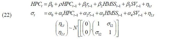
We assume that the same set of explanatory variables is the main factor that explains the variations in housing price volatility. To allow for the potential of a contemporaneous correlation between housing price changes and the corresponding volatility, the seemingly unrelated regression model (Zellner, 1962) is assumed. The empirical relationship between sentiment shock and housing price variables is further examined in the extended model shown in Eq. (22). This specification strategy is partially based on the theoretical model introduced in Section II.7
The other rationale for using the SUR is to consider housing price changes and volatility simultaneously with the same set of exogenous variables, as suggested by the theoretical model. Whereas previous studies mainly focused on the impacts of sentiment on housing prices, this study aims to examine not only its impacts on changes in housing prices but also its effects on housing price volatility. In this sense, the simultaneous equation approach (e.g., SUR) is considered to serve our research purpose better.8
(Baseline Model)
(Extended Model)
In these equations, HPC denotes the housing price change, r is the interest rate, HMSS is the housing market sentiment shock, SV denotes the sentiment volatility, σ represents the housing price change volatility, and σ12 is the correlation between housing price changes and the corresponding volatility.
This paper also aims to investigate whether the estimated sentiment shock has short-term predictive power in the future housing price index. The benchmark forecasting model for the comparison of the predictive power is set as the AR(1) model for housing price changes. The alternative predictive models incorporate housing market sentiment variables.
Benchmark Forecasting Model (AR(1)): β0 + ρHPCt-1 + et
Forecasting Model 1: β0 + β1HMSSt-1 + et
Forecasting Model 2: β0 + β1HMSSt-1 + β2SVt-1 + et
Forecasting Model 3: β0 + β1HMSSt-1 + β2SVt-1 + ρHPCt-1 + et
The forecasting models above predict the one-month-ahead housing price change based on currently available data. The RMSE (root mean squared error) is used as a key metric to compare the prediction accuracy rates of the forecasting models.
where h is the forecasting horizon, t is the time, and HP denotes housing prices.
In out-of-sample forecasting exercises, recursive forecasting and rolling-window forecasting are commonly used. In this study, both of these forecasting methods are applied and forecasting errors are compared across the two methods. Rolling-window forecasting is a method of deriving predicted values from an estimated model, with the window size fixed in the estimation of a forecasting model; that is, the number of samples is kept constant. On the other hand, recursive forecasting is a prediction method in which the sample period for the estimation is extended over time.9 The recursive forecasting method is expected to show better performance when the time series is stationary. However, when there are structural changes in the time series, the rolling-window prediction method is expected to be more advantageous.
In order to estimate the sentiment shock of the housing market, the monthly Housing Market Consumer Confidence Index (HMCI) published by the Korea Research Institute for Human Settlements is used. The housing price index provided by KB Real Estate, which represents the overall level of housing prices in the region, is used as a proxy for the housing price variable. In addition, the monthly mortgage interest rate compiled by the Bank of Korea is used in the estimation as a proxy for the interest rate in the estimation model.
To observe the effects of supply-side information on housing prices, new housing construction projects, in terms of the number of housing units, as authorized by the government are included in the extended model. This variable is considered to be one of the most important leading indicators of the housing supply cycle. As currently authorized housing construction projects go through the stages of sales, construction, and completion, such projects will lead to an actual housing supply increase in two to three years. As this variable is expected to act as an important factor related to housing purchases or investment decisions from the perspective of households, we included it as one of the determinants of housing prices in the extended model.10
The sample period used for estimating the empirical models is limited, ranging from January of 2011 to August of 2021. This period is selected in consideration of the time when the housing market consumer confidence index first began to be released. In addition, the period for which this study intends to predict through the out-of-sample forecasting ranges from September of 2017 to August of 2021. The summary statistics of the data used in the model estimation are shown in Table 1. In the HMSS case, the normalized variable is used in the model estimations.11 In addition, the number of new housing construction projects is log-transformed in the estimation of the extended model.
Note: 1) The mortgage interest rate is in a percentage form, 2) The sentiment shock is estimated from the regression of HMCI on the past housing prices changes (up to 12 months), 3) The number of new housing constructions is log-transformed, 4) The sentiment shock volatility is inferred from the GARCH(1,1) estimation of sentiment shock, 5) The housing price change volatility is inferred from the GARCH(1,1) model of housing price changes.
In this section, we report and discuss the key results of the estimation models. Given that our focus is on the role of sentiment shock in shaping future housing prices and on the corresponding volatility, our discussion centers on the HMSS and the SV.
We examine the effects of sentiment shock and sentiment shock volatility in the framework of seemingly unrelated regressions for two regions: (1) nationwide housing prices (2) those in the Seoul Metropolitan Region.12 Columns (a) in Table 2 and Table 3 show the estimation result of the baseline model, which excludes sentiment-related variables. The baseline model’s results suggest that there exists a momentum effect in housing price changes both at the national level and at the SMR level, given that the autoregressive term is found to be highly persistent. This result is consistent with numerous empirical studies that provide evidence of the existence of a momentum effect in returns on residential real estate (e.g., Case and Shiller, 1989; Beracha and Skiba, 2011).
Note: 1) *** p <0.01, ** p <0.05, * p <0.1, 2) HPC=housing price change, HMSS= housing market sentiment shock, SV=sentiment volatility, IR = interest rate, NC = number of newly permitted housing construction projects in terms of housing units, 3) Values in parentheses denote standard deviations, 4) The values in the parentheses in the correlation panel show the test statistics (Chi-square) of Breusch-Pagan test of independence among errors in the two regression equations.
Note: 1) *** p <0.01, ** p <0.05, * p <0.1, 2) HPC=housing price change, HMSS= housing market sentiment shock, SV=sentiment volatility, IR = interest rate, NC = number of newly permitted housing construction projects in terms of housing units, 3) Values in parentheses denote standard deviations, 4) The values in the parentheses in the correlation panel show the test statistics (Chi-square) of Breusch-Pagan test of independence among errors in the two regression equations.
The lagged term of housing price changes is also positively associated with the one-month-ahead volatility of national housing price changes and SMR housing price changes. As expected, the mortgage interest rate is found to depress one-month-ahead housing price changes. Furthermore, the interest rate is found to be positively associated with housing price volatility of the SMR.
The impact of the interest rate on housing price changes is fairly well in line with our intuition, given that higher interest rates are likely to translate into higher funding costs for leveraged investments in residential assets. On the other hand, the positive association between interest rates and housing price volatility for the SMR can be understood in the following context. First, note that higher volatility means there are more probable extreme outcomes in a random variable over its probability distribution. If higher interest rates can negatively affect the cash flows of highly leveraged investors, stressed investors likely wish to liquidate their purchased residential assets at more discounted prices, which may result in a major swing in housing prices. In the same vein, as lower interest rates are usually driven by high amounts of liquidity in the banking system, available mortgage loans in sufficient amounts can create an environment in which investors become more willing to pay high premiums, subsequently resulting in a large upside swing in housing prices.
Column (b) in Table 2 provides supporting evidence of the importance of the sentiment shock in determining housing prices and the corresponding volatility at the national level, indicating that a rise in sentiment shock positively affects housing prices in the subsequent period. Specifically, if sentiment shock increases by one standard deviation, one-month-ahead housing prices at the nationwide level then tend to rise by 0.054 percentage points, with the corresponding volatility tending to decrease by 0.042 percentage points.
Similar results are found in the SMR case: column (b) in Table 3 shows that an increase in sentiment shock predicts a positive housing price change for the SMR: a one standard deviation increase in sentiment shock predicts a positive move in the SMR’s housing prices by approximately 0.18 percentage points. However, unlike the results at the nationwide level, the sentiment shock here is found not to be statistically significant with regard to housing price volatility for the SMR.
Columns (c) in Table 2 and Table 3 show the results of the SUR estimation, in which sentiment shock volatility is considered. While the significance and direction of sentiment shock itself remain unchanged in this specification, we find no statistically significant links between sentiment volatility (SV) and housing price changes (HPC) at all regional levels.
Regarding the relationship between sentiment volatility and housing price volatility, column (c) in Table 3 shows that the volatility of sentiment shock is a significant determinant of the one-month-ahead housing price volatility at the SMR level, a finding in line with the predication of the theoretical model in Section III. However, at the national level, sentiment volatility is found not to be associated with housing price volatility, as shown in column (c) in Table 2.13
There are many different channels through which sentiment volatility can affect housing price volatility. One possible channel for this result being held is that if a householder’s subjective evaluation of residential real estate is inherently exposed to any sort of sentiment shock, either being fundamentally relevant or pure noise, his investment decisions on housing assets can become a function of sentiment shock. Thus, the aggregate demand for housing can become more volatile as sentiment shock becomes more volatile.
Furthermore, we also find that no statistically significant contemporaneous correlation between housing price changes and price volatility (denoted as σ12 in Eq. (21)) exists at either level, except for the baseline model at the national level. As we extend the model by adding sentiment-related variables, the statistical significance of the contemporaneous correlation between housing price changes and the corresponding volatility vanishes.
To check the impact of the supply-side factor, we augment the estimation model with the number of housing construction projects newly authorized by the government. Columns (d) in Table 2 and Table 3 show the results of the extended model after this augmentation. The significance of the supply-side information differs by region. While the significance of the sentiment-related variables is not substantially altered in this specification, column (d) in Table 2 shows that the increase in new residential construction projects authorized in the previous month is negatively associated with housing price changes and the corresponding volatility at the nationwide level, implying that more news about a substantial increase in the future aggregate housing supply can stabilize housing prices both in terms of the level and volatility.
Residential construction projects permitted do not immediately materialize into a dramatic increase in the aggregate housing supply in the subsequent months over such a short horizon. However, this finding suggests that news of a positive supply shock on the aggregate housing stock can be a stabilizing factor for the current housing market at the nationwide level in the short run.
However, surprisingly, this type of relationship is not observed in the SMR. This is attributable to the belief of many market participants that increases in the housing supply in the SMR would be substantially limited by geographical limitations and various government regulations. Furthermore, the robust demand in that region caused by the demographic concentration in the SMR may reinforce this belief, which can outweigh the positive supply shock on the housing stock. Otherwise, this result can be attributed to the fact that this supply-side variable (NC) represents the expected future housing supply at the national level, not at the SMR level.
In this section, we report the results of out-of-sample forecasting exercises for the forecasting models discussed in Section IV. The simple linear forecasting model for housing price uses only the sentiment shock variable. With the estimated parameters from the forecasting model, we produce out-of-sample forecasts for the housing price index at the national level and the SMR level.
As explained previously, we utilize two types of forecasting methods for each regional basis: the recursive method versus the rolling-window method. The realized housing price indexes along with predicted housing prices are plotted in Figure 5 and Figure 6. These figures demonstrate that this very simple forecasting model can generate out-of-sample forecasts which seem to capture well the overall evolution of historical housing prices.14
Note: 1) The dash-dotted line denotes the forecasted values, while the small dotted lines denote the 95% confidence interval of the forecasts, 2) The solid line denotes the actual housing prices, 3) These forecasts are produced by Forecasting Model 1.
Note: 1) The dash-dotted line denotes the forecasted values, while the small dotted lines denote the 95% confidence interval of the forecasts, 2) The solid line denotes the actual housing prices, 3) These forecasts are produced by Forecasting Model 1.
To gain a better understanding of the predictive power of the sentiment shock variable as proposed in this paper, we compare the prediction accuracy, in terms of the RMSE, of several forecasting models in Table 4 and Table 5. In the two forecasting methods, the prediction model equipped with the sentiment shock (HMSS) and the sentiment volatility (SV) variables outperforms the benchmark models. Furthermore, the forecasting model with only the sentiment shock variable (Forecasting Model 1) outperforms the benchmark forecasting models in all cases.
Note: HPC = housing price change, HMSS = housing market sentiment shock, SV = sentiment volatility, IR = interest rate.
Note: HPC = housing price change, HMSS = housing market sentiment shock, SV = sentiment volatility, IR = interest rate.
Interestingly, adding the lagged housing price change variable to Forecasting Model 2 is found to deteriorate the prediction accuracy over the out-of-sample periods.15 One possible rationale behind this result is that the HMSS may capture a sufficient amount of information that has already been incorporated into the lagged housing price such that no additional information can be gained.
In addition, we observe that the rolling-window forecasting method outperforms the recursive forecasting method for the housing price index at the national level for all prediction models considered here. However, for the housing price index of the SMR, the prediction performance varies depending on the model across the two forecasting methods.
This paper provides empirical evidence that sentiment shock can play an important role in shaping the dynamics of housing prices in the short run, and it also shows that volatile movements in market participants’ sentiment levels with regard to the housing market can contribute to the destabilization of housing prices, especially in the Seoul Metropolitan Region.
Though this paper does not deal with all aspects of the housing market in Korea, the key results of this study offer several important policy implications, specifically that attenuating household sentiment in the housing market can serve as an operational tool for stabilizing housing prices. Furthermore, consistency of housing-related policies is of great importance given that volatile housing prices are closely related to volatile sentiment. When formulating housing-related policies, policymakers must have projections on how those policies may affect the overall sentiment level of market participants and must have specific policy tools to manage sentiment such that they achieve their policy goals.
If the government's primary policy goal is to stabilize housing prices16, which have risen significantly in recent years, the government should be able to send consistent signals, in the form of specific regulations and policies, that the expected return on residential assets will not be abnormally high.
In addition to the demand-side management of sentiment, this study suggests that supply-side policies must also be pursued to stabilize housing prices, as knowing that the future housing supply will be significantly limited, market participants may maintain positive sentiment toward the housing market, even when they face various policies aimed to degrade overall sentiment in the housing market.
In this appendix, we report the results of the estimation model under different specifications when estimating the HMSS in Eq. (1) and the volatility of the HMSS. Specifically, the HMSS is derived from the regression in which the HMCI is regressed over the last six-month housing price changes. The volatility of the HMSS (denoted as SV) is estimated under different GARCH specifications.17
In Table A1 and Table A2, we only report the estimated parameters for the HMSS and the SV due to limited space here. The sign and the statistical significance of the HMSS remain unchanged at the national level. However, under the GARCH (2,1) and GARCH (2,2) specifications, it is found that sentiment volatility (SV) has a positive leading relationship with housing price volatility at the national level, which provides more supportive evidence of the importance of the sentiment volatility compared to the baseline specification.
Note: 1) *** p <0.01, ** p <0.05, * p <0.1, 2) HPC=housing price change, HMSS= housing market sentiment shock, SV=sentiment volatility, 3) Values in parentheses denote standard deviations, 4) In these estimations, HMSS is derived from the regression in which the HMCI is regressed over the past six months of housing price changes.
Note: 1) *** p <0.01, ** p <0.05, * p <0.1, 2) HPC=housing price change, HMSS= housing market sentiment shock, SV=sentiment volatility, 3) Values in parentheses denote standard deviations, 4) In these estimations, HMSS is derived from the regression in which the HMCI is regressed over the past six months of housing price changes.
On the other hand, at the SMR level, the results under alternative specifications are consistent with those of the baseline specification.
The study simply counts the number of predefined positive words against predefined negative words in the abstracts of news articles.
For example, it is less expensive to construct the index. In addition, the index can be constructed in a timely manner.
We confirm that the HMCI is a stationary time series, as shown in the following ADF (augmented Dickey-Fuller) test results.
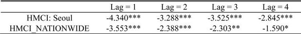
Note: *** p<0.01, ** p<0.05, * p<0.1.
The momentum effect refers to the tendency of an asset price to increase (decrease) further if it has increased (decreased) in the past periods.
Note that the specification of the extended model is set to approximately capture, in discrete time, the equilibrium relationship between housing price changes and housing price volatility in the presence of sentiment bias in households’ expectations.
While the VAR and VECM may be other candidates for analyzing the short-run dynamics of housing prices, in such cases we must devise an additional regression equation for housing price volatility. While we can also investigate the impact of sentiment shock using the VAR framework, the SUR is more in line with the theoretical framework we established here.
That is, with recursive forecasting, the number of samples continues to increase in the estimation stage of the prediction model as time elapses, whereas for rolling-window predictions, the number of samples for the estimation of the prediction model remains constant.
One disadvantage of this variable is related to how it provides information about the expected future housing supply considering that such outcomes are not equivalent to the actual supply of housing. However, if we assume that households utilize all available information when they make decisions at the current time, we can consider that this variable captures supply-side information of the housing market.
Note that the nationwide housing price index covers all regional areas of South Korea, including the Seoul Metropolitan Region. Thus, those two price indices are closely related, given that the SMR makes up a large proportion of housing market capitalization in Korea.
However, under different GARCH specifications on the SV, the SV is positively associated with the volatility of housing prices at the national level, as shown in Appendix A.
In Appendix B, we provide the figures of the out-of-sample forecasts on housing price changes, from which the forecasts of housing price levels are computed.
Note that having more explanatory variables in the forecasting model does not always lead to better prediction accuracy in forecasting exercises in various settings.
Though it takes more work to gauge the level of housing prices so as to conclude the presence of a housing bubble, the fact that the normalized housing price (i.e., housing price to income ratio) in the Seoul Metropolitan Area is substantially higher than those of major cities in other comparable countries warrants further investigation. The rigorous econometric test of the existence of a housing bubble in Korea is left for future research. Some argue that such a housing bubble can create many economic and social problems, including record-low birth rates, stagnant domestic consumption, and social inequality. The empirical relationships between housing prices and related economic/societal problems should be thoroughly examined. The effects of housing prices on consumption and the fertility rate may differ depending on the status of homeownership, as pointed out by Campbell and Cocco (2007). The most worrisome aspect of such a housing bubble is that the consumption profile of an ordinary household living in a city with abnormally high housing price appreciation may not be consistent, even after considering the bequest motive, with the intertemporal-utility-maximizing consumption profile. This can lead to a failure to achieve consumption smoothing over the life cycle.
, & . (2006). Investor sentiment and cross-section of stock returns. Journal of Finance, 61(4), 1645-1680, https://doi.org/10.1111/j.1540-6261.2006.00885.x.
, , & . (2012). Global, Local, and Contagious Investor Sentiment. Journal of Financial Economics, 104(2), 272-287, https://doi.org/10.1016/j.jfineco.2011.11.002.
, & . (2011). Momentum in Residential Real Estate. Journal of Real Estate Finance and Economics, 43, 299-320, https://doi.org/10.1007/s11146-009-9210-2.
, , & . (2019). On the Relationship between Market Sentiment and Commercial Real Estate Performance—A Textual Analysis Examination. Journal of Real Estate Research, 41(4), 605-638, https://doi.org/10.22300/0896-5803.41.4.605.
, & (2007). How do House Prices Affect Consumption? Evidence from Micro Data. Journal of Monetary Economics, 54(3), 591-621, https://doi.org/10.1016/j.jmoneco.2005.10.016.
, & (2003). Is There a Bubble in the Housing Market? Brookings Papers on Economic Activity, 2003(2), 299-342, https://doi.org/10.1353/eca.2004.0004.
, , & . (2007). Sports Sentiment and Stock Returns. The Journal of Finance, 62(4), 1967-1998, https://doi.org/10.1111/j.1540-6261.2007.01262.x.
, , & . (2018). News-based sentiment analysis in real estate: a machine learning approach. Journal of Property Research, 35(4), 344-371, https://doi.org/10.1080/09599916.2018.1551923.
, , & . (2005). Assessing High House Prices: Bubbles, Fundamentals and Misperceptions. The Journal of Economic Perspectives, 19(4), 67-92, https://doi.org/10.1257/089533005775196769.
, & . (2021). News Media Sentiment and Asset Prices: Text-mining approach. Asia Pacific Journal of Accounting and Economics, 28(2), 183-205, https://doi.org/10.1080/16081625.2019.1642115.
(2018). Quantifying Sentiment with News Media across Local Housing Markets. The Review of Financial Studies, 31(10), 3689-3719, https://doi.org/10.1093/rfs/hhy036.
. (2021). House Price History, Biased Expectations, and Credit Cycles: The Role of Housing Investors. Real Estate Economics, 49(4), 1238-1266, https://doi.org/10.1111/1540-6229.12328.
. (2007). Giving Content to Investor Sentiment: The Role of Media in the Stock Market. Journal of Finance, 62(3), 1139-1168, https://doi.org/10.1111/j.1540-6261.2007.01232.x.
, , & (2008). More than Words: Quantifying Language to Measure Firm Fundamentals. Journal of Finance, 63(3), 1437-1467, https://doi.org/10.1111/j.1540-6261.2008.01362.x.
. (2014). Housing Booms and Media Coverage. Applied Economics, 46(32), 3954-3967, https://doi.org/10.1080/00036846.2014.948675.
. (1962). An Efficient Method of Estimating Seemingly Unrelated Regressions and Tests for Aggregation Bias. Journal of the American Statistical Association, 57, 348-368, https://doi.org/10.1080/01621459.1962.10480664.
, & . (2021). Housing Price Dynamics: The Impact of Stock Market Sentiment and the Spillover Effect. The Quarterly Review of Economics and Finance, 80, 854-886, https://doi.org/10.1016/j.qref.2019.02.006.
, , & . (2016). Investor Confidence as a Determinant of China's Urban Housing Market Dynamics. Real Estate Economics, 44(4), 814-845, https://doi.org/10.1111/1540-6229.12119.