- P-ISSN 2586-2995
- E-ISSN 2586-4130

This paper analyzes job creation when the Korean economy transitioned to a knowledge economy from the 1990s to the 2010s. During this period, the ratio of service to manufacturing jobs increased, knowledge intensive industries grew, and job creation became geographically concentrated around Seoul. The changes slowed down in the 2010s, and overall job growth weakened. To analyze the effect of job creation driver industries during this period, the main part of which are knowledge intensive tradable service industries, on local service job creation, I use a modified version of the local labor market of Moretti (2010). I analyze the job changes during 1995-2005 and during 2006-2016 in 237 Si-Gun-Gu areas in the Census on Establishments datasets. I find that one manufacturing job creates 0.5 local service jobs and that one tradable service job creates 1.1 jobs within Gu areas of metro cities and 2.3 jobs in Si-Gun areas. The job creation relationship between the tradable and local service sectors was not altered in this period. As more jobs were created in the tradable sector driven by the transition to a knowledge economy, job creation overall remained active, with the opposite also being true.
Korea, Job Creation, Local Labor Market Model, Knowledge Economy
J01, J21, J23, J24, R11, R12
Job creation has emerged as a top-priority policy goal in Korea such that the incoming government referred to itself as a ‘Jobs Government’ in 2017.1 Figure 1 presents Korea’s employment trend on a log scale from 1995 up to 2020.2 Korea has overcome two major economic crises, in 1998 and in 2008, and sustained its job growth path, but job growth has weakened noticeably during the last decade. There were heated debates over the proper strategies to use for job creation in 2017. This research is motivated by these debates.
Note: Natural log of all industry workers in thousands.
Source: Korea Statistics, Economically Active Population Survey.
The Korean economy has been a typical manufacturing economy, and its comparative advantage has shifted from low wages to technology over the past few decades. At the same time, the driving force of job creation has moved from manufacturing to knowledge industries. The objective of this paper is to show how jobs were created during the transition to a knowledge economy in Korea in the period from the mid-1990s to the 2010s.
Labor demand functions presume a stable relationship between output and labor requirement and derive labor demand levels from production. However, in a knowledge economy, knowledge-intensive jobs in the tradable sector create more jobs outside the sector through job creation spillover effects.3 The labor demand framework does not take into account these job-creation effects, because it derives the amount of labor needed for production, which is a rather small percentage in its total job-creation effect. Input-output tables calculate labor requirement in related industries. They do not address the spillover effects on unrelated industries. Thus, I use a local labor market job creation model, suggested by Moretti(2010), to analyze job creation during this transition period. This framework divides the economy into two sectors: the tradable sector and the non-tradable sector. Jobs in the tradable sector are created when they are productive enough, while jobs in the non-tradable sector are created by the spillover effects of job in the tradable sector. This paper addresses how the tradable sector changed as the economy transitioned to a knowledge economy and how the spillover effect acted during this period.
This paper has two parts. In the first part, Section II, I address the question of how one can infer that there has been a job creation mechanism change in Korea. The answer to this question is naturally related to the issue of how the tradable sector changed as the Korean economy transitioned to a knowledge economy. There have been conspicuous changes, such as the ratio of service to manufacturing jobs, geographical job creation patterns, and the growth of knowledge-intensive industries. One question long in the author’s mind concerns why more jobs are created when manufacturing jobs decrease. This question cannot be answered if the decrease in the number of manufacturing workers is accompanied by a transformation of manufacturing and an increase in knowledge-intensive industry workers, and the latter has a larger spillover effect. Topics in Section II may appear to be less interrelated; nonetheless, the author had this question in mind.
The second part, in Sections III and IV, addresses the question of how the spillover effects changed during this transition period. In order to answer this question, I introduce the local labor market model in Section III and show how the elements are constructed along with their trends. Section IV performs a regression analysis of the model proposed in Section III and discusses the estimation results.
This research has the following policy implications. If both the strong job creation in the 2000s and its weakening in the 2010s are related to the growth of knowledge-intensive industries, which are closely related to manufacturing, which policies affect their sustained growth? There are many proposals in the literature domestic and abroad, but further investigations of our own problem appear to be necessary. According to the model in this paper, local services such as restaurants and small shops have little spillover effects on other industry jobs, allowing room to manoeuver by policymakers on issues such as protection of traditional markets and the minimum wage, among others. Section V presents the summary and conclusion.
At an early stage of economic development, manufacturing usually serves as the major driving force of job creation. As the economy matures, this role moves to the service industries. Table 1 and Figure 2 show the numbers of manufacturing and service jobs and their ratios between 1970 and 2020. The 1970s and 1980s represented an industrialization and growth spurt era for Korea. The number of manufacturing jobs nearly doubled in a decade, as indicated by the dotted line in Figure 2. For each manufacturing job, two service jobs were created in a parallel fashion such that the ratio between the two remained around 2.0 in this period (Table 1, row 3). From the 1990s, service jobs continue to grow without being accompanied by manufacturing job growth. Consequently, the ratio rises, reaching 4.5 in 2010. Afterwards, the rise becomes stagnant and overall job growth weakens.
Note: Service is all industry except for agriculture, quarrying, mining, and manufacturing.
Source: Author’s calculation from Korea Statistics, Economically Active Population Survey.
Source: Author’s calculations from Korea Statistics, National Accounts, GDP by Economic Activities.
The growth of service jobs in the 1990s and 2000s suggests that some force other than manufacturing may have driven job creation. This shift is the main subject of this paper. On the production side, noticeable is the growth of knowledge-based industries in this period. The growth of knowledge-based industries is one of the major changes that occurred in advanced economies in the late 20th century.4 The OECD notes that ‘economies are increasingly based upon information and knowledge as drivers of productivity and growth’ (OECD, 1996, p.3). The quantitative content of this claim is the rising share of knowledge-based industries, which are technology-intensive manufacturing and knowledge-intensive service industries, in overall output. The OECD report further notes, “Indeed, it is estimated that more than 50 percent of Gross Domestic Product (GDP) in the major OECD economies is now knowledge-based” (p.9).5
In the literature, knowledge-based industries are broadly defined without a single consensus. Cermeño (2018) observes that the share of knowledge-based business services (KIBS) in GDP increased consistently over the very long period of 1950 to 2010. Cermeño (2018, Figure 1, p.146) shows that its share rose from 18 percent in 1950 to 35 percent in 2010, while the shares of manufacturing and non-KIBS service remained basically stagnant, hovering between 10 to 15 percent. Her definition of KIBS is very broad and includes finance and insurance, real estate, business services, and professional services.6
In order to review a corresponding trend in Korea’s context, I need a definition of knowledge-based industries. The OECD STI (Science, Technology and Innovation) directorate regularly updates the list of technology-intensive manufacturing and knowledge -intensive service industries in its STI scoreboard publication.7 I classify high-tech and medium-high-tech industries as technology-intensive manufacturing industries.
The series of long-run value added by industry in Korea’s National Account System is available from 1970 in 13 manufacturing and 21 service industries.8 I regard the following as tech-intensive manufacturing: chemicals (including pharmaceuticals); computers; electronic and optical instruments; electrical equipment, machinery and equipment; and transport equipment (motor vehicle and other transport). With regard to knowledge-intensive services, I select financial and insurance, information and communication, business services, and education. The health industry is clearly knowledge intensive but it is bound together with social work in the output statistics. Therefore, I separate out this industry.
Table 2 shows the shares of technology- and knowledge-intensive industries out of total value added in five-year intervals between 1985 and 2020. The first row is the share of manufacturing, and it remains between 27 and 30 percent throughout in the past 35 years. However, within manufacturing, the share of technology-intensive industries consistently rises up to 2010.9 This trend is graphically shown in Figure 3 over a longer horizon. This rise explains the gap between the constant output share and the falling employment share of manufacturing. The share of KIBS rises faster than the share of tech-intensive manufacturing. Starting from a similar level, the share of KIBS stands above that of tech-intensive industries in 2010 as a consequence of its quicker ascent in the 1990s and 2000s. The increase would have been quicker if medical services were added to it. Again, it flattens from 2010 onwards. When tech-intensive industries, KIBS, and health and social work are considered as knowledge-based industries, the sum of their shares reaches 48.2 percent as of 2020, slightly below one half (row 4).
Note: KIBS industries are financial and insurance, information and communication, business services, and education. Knowledge-based is the sum of tech-intensive, KIBS and health, social work values.
Source: Author’s calculations from Korea Statistics, National Accounts, GDP by Economic Activities.
Note and Source: Identical to that in Table 2.
Another important evidence indicating a shift in the job creation pattern is the geographical concentration of job creation areas. Figure 4 compares the locations of the top 10 job creation Si-Gun-Gu areas in the decade from 1995 to 2005 with those in the decade from 2006 to 2016. The sizes of the circles are proportional to the numbers of jobs created. In the previous decade, the areas were either new residential areas or manufacturing centers located along the Seoul-Pusan line (See Column 3 in Table 3). In the latter decade, all are within or near the Seoul metropolitan area. Some are new residential areas but the majority are knowledge-intensive service industry centers. Clearly, job creation has gravitated towards Seoul, especially to the Gangnam area, which is the new and prosperous part of Seoul. Among the three Gu’s in the Gangnam area, one is ranked at the second and another is at the fourth place. The Gu at the fifth is bordering with the Gangnam.
Note: The sizes of circles are proportional to the number of jobs created.
Source: Author’s calculations from the Korea Statistics, the Census on Establishments, micro datasets.
Note: 1) * Percent of workers in manufacturing in all industries exclusive of agriculture, fishery, quarrying, and mining, 2) ** Average of Gyeonggi Goyang-si.
Source: Author’s calculations from the Korea Statistics, the Census on Establishments, micro datasets.
Table 3 lists the names of the top 10 areas in Figure 3. The administrative district units are Si-Gun-Gu. A ‘Gu’ is a district within a large city. It corresponds to, for example, a borough in the U.S. A ‘Si’ is a small to medium-sized city which does not belong to a metropolitan area. A ‘Gun’ is a district in less urbanized areas. There are approximately 250 Si-Gun-Gu areas in Korea with an average population size of around 200 thousand.
A detailed review of the new jobs in the Gangnam area by industry reveals that the majority are professional service jobs such as business headquarters, legal service, and programming jobs (See Table 4). These jobs are knowledge intensive and have agglomeration effects. Hence, the geographical concentration is interpreted as a consequence of the transition to a knowledge-based economy. Knowledge activities in highly complicated industries are very specialized such that cooperation becomes important and participators congregate in specific areas (Balland et al., 2008). As these effects are strong at very short distances, such as within miles, knowledge industries tend to be highly concentrated geographically (Rosenthal and Strange, 2004).
Knowledge-intensive services mean that the service industry requires a high level of knowledge activity for production or delivery of the services. The OECD classifies knowledge-intensive services according to the share of the highly educated among the workers in the industry. The OECD classifies this at the two-digit level. In ISIC3, communication (64), financial and insurance (65, 66, 67), and business support (71-74, excluding real estate) belong in this category. Education (80) and health (85) are intermediate, and they are usually categorized separately.10
The NSB (National Science Board, 2018) uses a more detailed classification and excludes some service industries that do not require a high level of knowledge activity. For example, it excludes social work and the renting of household goods (713, in ISIC3 henceforth). This classification takes into account the level of R&D intensity in services and includes the publishing of recorded media (221) and news agency activity (922) as knowledge-intensive services. Since the OECD classifies this at a two-digit level and both health and social work are in ISIC3 85 industries, social work is classified as knowledge intensive as health is an important knowledge-intensive service. However, social work is not treated as knowledge-intensive when a lower level of classification is used, as done by the NSB.
The countrywide version of the Census on Establishments datasets contains industrial classification codes up to five digits.11 I select five-digit industries corresponding to ISIC3 classification 71 (renting of machinery and equipment, household goods), 72 (information, computers), 73 (R&D), 74 (professional, scientific, and technical services), 65-67 (financial, insurance), 642 (communication), 80 (education), and 851(medical), and exclude rentals of consumer goods (713) and include the publishing of recorded media (221) and news agency activity (922). This result is shown in Figure 5.
Source: Author’s calculations from Statistics Korea, Census on Establishment micro datasets.
The share of knowledge-intensive service workers among all industry workers rises robustly from 1995 to the end of the 2000s and then levels off. The rise is sharpest in the 2000s. Industrial classification codes were revised between 2005 and 2006, but a break is not apparent.
The trends shown in Figures 1 to 5 are all interrelated. The Korean economy’s transition to a knowledge economy was rapid in the 2000s, and both technology-intensive manufacturing and knowledge-intensive services grew rapidly. Knowledge-intensive services played an important role in job creation, and jobs became concentrated within or near the Seoul metropolitan area. As the pace of the transition decelerated, job creation weakened. The next section focuses on the spillover effects of the knowledge sector on non-tradable, local service jobs.
This section establishes a local labor market model to estimate the job-creation effects of a knowledge economy. An important feature of a knowledge economy is its geographical concentration. By comparing localities where knowledge industries are concentrated with those in which they are not, a meaningful inference about the job-creation effects can be made. This is one of the reasons why a local labor market model is particularly useful when analyzing a knowledge economy. Another advantage is that one can disregard institutional effects, which often complicate a labor market analysis, as localities within a country have largely the same institutions.
On the other hand, an international comparison or an input-output analysis is not appropriate in this context because between countries there are wide differences in institutions whereas their stages of transition towards a knowledge economy are similar. An I-O model presumes a national economy and quantifies transactions between industries. On a national scale, one cannot identify the effects of a knowledge sector on local service job creation. Moreover, definitions of knowledge or tradable industries are not so clear-cut such that detailed industry information is needed, but I-O sectors are defined broadly for data reasons. General equilibrium aspects such as rising housing prices at knowledge centers cannot be addressed either.12
This section is organized as follows: Subsection A builds a local labor market model, subsection B discusses how to determine local labor markets, subsection C defines tradable services, and finally subsection D compares tradable services with knowledge-intensive services.
I set up a simple local labor market model to estimate job creation in a knowledge economy. A local labor market model presumes two sectors within an economy―the tradable sector and the non-tradable sector, which is equivalent to the local service sector. The sectors are divided based upon industry characteristics. The tradable sector does not exactly overlap with knowledge-intensive industries, but as the tradable sector growth is driven by knowledge industries, the effects of its growth virtually reflect the effects of knowledge-sector growth.
Goods and services in the tradable sector are produced to meet outside demands, while services in the non-tradable sector are produced locally to meet local demands. Typical tradable sector industries are manufacturing and agriculture, where goods are traded to meet outside demands. There are service industries in the tradable sector as well, and they are called ‘tradable services.’ They are usually professional and knowledge-intensive services, such as broadcasting, universities, medical hospitals, and legal services, among others. The industries in the non-tradable sector are local services by nature, such as restaurants, lodging establishments, retail shops, laundry and cleaning businesses, construction companies, medical clinics, and primary schools. Local services are mostly not highly knowledge intensive, but there are exceptions, such as clinics and schools. However, they do not constitute the main growing part in a knowledge economy.
The model I use is a modified version of Moretti (2010) with the results of Van Dijk (2015; 2018) taken into consideration. The basic model is as follows:
In equation (1), the superscript NT denotes the non-tradable sector. Unlike in Moretti (2010), the tradable sector consists of two parts: manufacturing (T1) and tradable services (T2). Figure 4 and Table 3 provide a hint of the rising importance of tradable services as a driver of job creation, and I choose to separate the two. Primary industries (agriculture, fishery, forestry, and mining) are dropped from the sample throughout.
The subscript c denotes city, which corresponds to a ‘Si-Gun-Gu’ in this study, and t is time, which is a ten-year period. The variable L represents the number of jobs in the sector. The growth rates of L are defined using the initial period total, 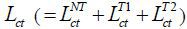 as denominators. The reason I use the total instead of its own initial period value
is to control excessive volatility.13 Local labor markets are small and the growth rates tend to vary widely when their
own initial values are used.14 For example, when a plant moves out from inside a city to its vicinity, the city’s
manufacturing employment growth rate then shows a large negative number while that
of the affected vicinity becomes very large, magnifying the estimation error. The
initial period total suppresses such large variations. Van Dijk (2015) performs a sensitivity test and recommends the use of linear differences over the
total as growth rates. The variable Cct is a set control variables for area characteristics. I use the shares of those educated
at a four-year university or more among the population aged between 25 and 64 in the
Population and Housing Census data. Dummies for metropolitan areas are not used as
they are statistically insignificant. A full fixed-effect model is not used, as in
this case I lose one of the two periods.
as denominators. The reason I use the total instead of its own initial period value
is to control excessive volatility.13 Local labor markets are small and the growth rates tend to vary widely when their
own initial values are used.14 For example, when a plant moves out from inside a city to its vicinity, the city’s
manufacturing employment growth rate then shows a large negative number while that
of the affected vicinity becomes very large, magnifying the estimation error. The
initial period total suppresses such large variations. Van Dijk (2015) performs a sensitivity test and recommends the use of linear differences over the
total as growth rates. The variable Cct is a set control variables for area characteristics. I use the shares of those educated
at a four-year university or more among the population aged between 25 and 64 in the
Population and Housing Census data. Dummies for metropolitan areas are not used as
they are statistically insignificant. A full fixed-effect model is not used, as in
this case I lose one of the two periods.
The parameters β1 and β2 are the central parameters and measure how many non-tradable sector jobs an additional tradable sector job creates. For this reason, Moretti (2010) calls them ‘local multipliers.’15 These parameters reflect general equilibrium effects, which should be taken into account when interpreting estimates.16 For example, if there is a productivity shock in an area, it pushes up housing costs and reduces local service job-creation effects.
Another issue is whether to use weights in the estimations. I use the initial period total employment sizes Lct as weights. Moretti (2010) uses total employment sizes in 1990 as weights both for the 1980-1990 and 1990-2000 periods. Van Dijk (2018) recommends OLS instead. He explains that WLS and OLS estimates have different interpretations. OLS estimates the job-creation effect in an average area, whereas WLS estimates the effect of an average job. In the Census on Establishments sample, the sizes of Si-Gun-Gu areas are very diverse and metropolitan Gu areas are much larger. The WLS estimation is driven by large areas, whereas the OLS results are determined by many small areas. As tradable services are concentrated in large areas, and WLS produces larger 𝑅2 values, I choose to use WLS. As for the weights, population sizes can be alternatives, but as populations must be retrieved from the Census dataset17 and they exist in five-year intervals, I choose to use total worker sizes. Experimentation with population sizes as weights gives just slightly different results.
To implement the model, local labor markets must be determined among others. An obvious choice is a city. A city is a geographical unit composed of business centers and residential areas. Workers are much more mobile within a city than between cities. The difficulty of commuting produces housing price differentials across cities, which is a major reason of wage differentials between cities in a local labor market model.
The residential area of workers in a city is called a commuting zone (CZ), and a local labor market is commonly identified with a CZ. Commuting zones are determined from an travel-to-work pattern analysis in census data. Tolbert and Sizer (1996) selected 741 CZs in the U.S. using the U.S. Census data, which are commonly used in U.S. studies. For Korea, Yoon et al. (2012) at the Korea Labor Institute adopt the same method and construct 130 local labor markets using a 10% subsample of the Korea population and housing census data. They use Coombe’s algorithm, which determines zones from workers’ travel-to-work flows. In their construction, the entire Seoul metropolitan area plus some adjacent cities constitute a single local labor market, as the residences of workers in Seoul are very widespread geographically.
A problem with this construction is that the Seoul labor market covers a very large part of the Korean economy––one-fifth of the total population and a quarter of total production―which makes inference based on comparisons of local labor markets less meaningful. Furthermore, job concentration in the 2000s is towards the Gangnam area, which is located in the southern part within the Seoul metropolitan area, with a population size less than one-fifth that of Seoul.18 When the entire Seoul metropolitan area is regarded as a single labor market, job concentration within Seoul cannot be analyzed. Cermeño (2018) uses counties in the U.S. to analyze a century-long pattern of localization of job creation in the U.S. There were 3,143 counties in the U.S. as of 2010, and a county is a much smaller unit than a commuting zone. Cermeño finds that increasing returns-to-scale effects of a knowledge economy are a major cause of the job concentration effect in the 2000s in the U.S. As the increasing returns-to-scale effect is very sensitive to distance,19 she uses a smaller unit of areas.
As an alternative, I use a ‘Si-Gun-Gu’ as a local labor market. A ‘Si-Gun-Gu’ is the smallest administrative entity with local administration in Korea. A ‘Si’ is a small to medium-sized city that is not part of a metropolitan area. A ‘Gun’ is a district in a rural area. A ‘Gu’ is a district in a metropolitan city. There are six metropolitan cities, and Seoul has 25 Gu areas. As of the end of 2017, there were 260 Si-Gun-Gu in Korea.20 These consist of 75 Si, 82 Gun, and 69 Gu with local administrations and two other non-autonomous Si and 32 Gun. The Census on Establishment samples have 245 Si-Gun-Gu areas in 2000, 250 in 2005, 251 in 2010, and 250 in 2016. I use a version of the Census on Establishments data that has information on Si-Gun-Gu as well as Eup-Myon-Dong, which is a lower unit, and industrial classification codes up to three digits. Administrative districts have been reorganized several times, and I match the districts in the 1995 and 2005 and the 2006 and 2016 samples using Eup-Myon-Donginformation and each Si-Gun-Gu’s history on the Namuwiki websites.21 I drop very small districts so that the sample is composed of 237 Si-Gun-Gu areas. Many metropolitan Gu areas are adjacent, and job creation spillover effects may occur in other Gu areas. This can diminish spillover effect estimates, but I use the locations of establishments and not residences, and more importantly, if the entire Seoul area is a single labor market, I cannot address job concentration in a knowledge economy properly.
In equation (1), the tradable sector consists of manufacturing and tradable services. Tradable services constitute an important part given that the spillover effects are large. Job concentration in large cities cannot be explained without tradable services. By definition, the tradable sector is composed of industries that supply outside areas, but as transactions are not recorded, a different way of identifying tradable industries is needed.
Professional services such as broadcasting, advertising, universities, and hospitals are doubtlessly tradable in nature. Primary and secondary schools as well as local medical clinics are knowledge-intensive local services. Industries in financial services, communication, health, and education retain both tradable and non-tradable characteristics, and a clear-cut borderline is difficult to draw. Bank branches meet local demands but their headquarters function as a tradable service.
Jensen and Kletzer (2005) propose a simple way of identifying a tradable service. By definition, the sizes of local services are likely to be proportional to the area sizes in terms of population or employment. For tradable services, this is not necessarily the case. Thus, if an industry is geographically concentrated and its distribution is unrelated to the sizes of the areas, it can be regarded as a tradable industry. The measures of geographical concentration can be diverse, and Jensen and Kletzer (2005) use a locational Gini index. The index measures how unequally the industry workers are distributed compared with distribution of the population or employment. When the industry’s worker distribution is perfectly proportional to the population or employment distribution, the industry has a Gini value of zero, whereas when all workers in the industry are concentrated in a single area, its Gini value is one.
The version of the Census on Establishments dataset I use to estimate the local labor market model has detailed location information up to the Eup-Myon-Dong level but only three-digit industry codes. The three-digit classification information is adequate for dividing industries into tradable and non-tradable types. It distinguishes primary, middle, high schools, and colleges. Departments, supermarkets, and convenience stores are different industries. Use of very fine five-digit classification does not greatly improve the quality of the division. For example, bank branches and headquarters are in the same industry even at the five-digit level. One complication is that the Eup-Myon-Dong sample does not contain full observations, as Statistics Korea drops observations if there are two or fewer establishments in the same industry in the same area for confidentiality reasons. This omission impairs the accuracy of Gini indices. For this reason, I calculate the industry Gini indices from older version datasets that were produced before this omission rule has been implemented. I use the 2005 sample for KSIC8 and the 2010 sample for the KSIC9 classification.22
Regarding the choice of a threshold Gini index value, Jensen and Kletzer (2005) simply suggest guidelines. They report that Gini values of 0.1 and 0.3 divide the sample roughly into thirds. They recommend the choice of a threshold value that sets all manufacturing as tradable, construction as non-tradable, and the majority of public utilities as non-tradable.
The first and second rows in Table 4 show the shares of non-tradable sector workers for the threshold values 0.1 and 0.3 in the respective years. As in Jensen and Kletzer (2005), each constitutes approximately a third of the total. Typical local services such as haircuts, retail stores, restaurants, primary and middle schools, post offices, police and fire stations, and local administrative offices have Gini values of less than 0.1. Local medical clinics are usually located close to this threshold value. When the value is set to 0.3, the share of industries below the threshold is slightly less than 0.6. Jensen and Kletzer (2005) recommend the use of a public utility industry as a borderline industry. If I use water supply industry (360 in KSIC9) as the borderline,23 the shares of local service industries are approximately two-thirds, as given in row 3. In this classification, some public utilities, wholesale companies, long-distance transportation companies, certain financial and insurance services, colleges and special high schools, and movie and broadcasting companies are in the tradable sector.
Note: 1) Shares in all industries excluding primary industries. See text for definitions of sectors, 2) *Average of the three Gu areas (Seocho-gu, Gangnam-gu, and Songpa-gu).
Source: Statistics Korea, author’s calculations from Census on Establishment micro datasets.
In classifying industries into tradable and non-tradable types, I consider the industry characteristics in addition to the Gini value. Industries in the sections of business support (N), real estate (L), arts, sports, leisure (R), and associations and membership organizations (S) are local services by nature. Some of them are distributed very unevenly, such as labor unions (942), business support services (751), worker dispatch agencies (759) and real estate activity agencies (681). These industries meet local demands but because their customers are distributed unevenly, they are distributed unevenly. For example, labor unions are close to factories but factories are concentrated. Real estate activity agencies are concentrated where real estate transactions are active. These industries are classified as local services as jobs in the industries are created by spillover effects of other tradable industries. Some specialized services such as travel agencies (752) and security companies (753) are located at the centers of large cities. I classify them as tradable services.
The rows of row 4 and below show the sector’s shares by region. Countrywide, the shares of tradable services show a rising trend. This increase is strong in Seoul, and it is strongest in the Gangnam area. The trend for the non-Seoul areas rises very modestly, which is not shown here, but as can be inferred. The gaps in the trends explain job creation disparity between the Seoul metro area and others. Local services’ shares do not show any clear trends in all cases. The increase in the shares of tradable services is matched by the decline of manufacturing’s shares.
Tradable and knowledge-intensive services have different definitions and have different component industries, but their growth characteristics are common in a knowledge economy such that the effects of the tradable service sector growth reflects the effects of growth the knowledge sector. While a tradable service industry can be selected empirically, the definition of a knowledge-intensive industry is less clear-cut. This subsection reviews their relationship and show that tradable service growth is largely due to knowledge-intensive service growth.
Table 5 shows the composition of tradable and knowledge-intensive industries in the service industry for the years 1995, 2005, 2006, and 2016 and the corresponding changes. In column (4), the share of knowledge-intensive industries in the services rises from 0.21 in 1995 to 0.25 in 2016 (in rows 3, 6, 12, and 15).24 Within tradable services, its share rises much more quickly from 0.34 in 1995 to 0.59 in 2016 (rows 1, 4, 10, and 13).25 Such trend implies that the growing part of tradable services is likely to be the knowledge-intensive part.
Note: See the text for definitions.
Source: Author’s calculations from Statistics Korea, the Census on Establishments micro datasets.
Rows 7 to 9 and 16 to 18 show the changes in the ten-year periods. Between 1995 and 2005, tradable services increase by 322 thousand. Among them, the knowledge-intensive component accounts for 280 thousand, i.e., 87%. Between 2006 and 2016, tradable services increase by 1,204 thousand, with 819 thousand or 68% stemming from knowledge-intensive services. In addition to aggregate numbers, the high-tradable-service-growth areas are at the same time shown to be high-knowledge-industry-growth areas, as in the Gu areas in the Gangnam area. In the estimation, I use changes in the numbers of workers in the tradable and local service sectors and interpret the effects of tradable service growth practically as the effects of knowledge-intensive service growth.
Section IV reports and discusses the estimation results. In a local labor market model, tradable sector jobs create non-tradable sector jobs through the spillover effect. Actually, much more jobs are in the non-tradable sector than in the tradable sector. An estimation of the spillover effects will show how the job-creation mechanism has changed as the tradable sector grew and became more knowledge intensive.
I analyze the change in the 1995 to 2005 period (in KSIC8) and in the 2006-16 period (in KSIC9) from the Eup-Myon-Dong level and three-digit version of the Census on Establishments samples. A ten-year period is a natural choice as spillover effects take a very long time to fully materialize. 26 I drop agriculture, fishery, forestry, and mining from the sample. The weight variables are the number of workers in all industries (excluding primary industries) at the initial periods, in 1995 and in 2006.
The sample consists of 237 Si-Gun-Gu countrywide. There are 25 Gu in Seoul, 43 Gu in five other metropolitan cities, and 169 Si-Gun, which are composed of basically small to medium-sized cities. Table 6 shows the sample summary statistics. An average Gu in Seoul has 155 thousand workers, twice as large as an average Gu in other metro areas which is 89 thousand workers. These are again twice the size of an average Si-Gun, which has 43 thousand workers. Although there are much more Si-Gun areas in the sample, a Gu is much larger, consequently the totals of all Si-Gun and all Gu are approximately of the same size. The numbers of manufacturing workers increase in Si-Gun but decreases in metropolitan Gu areas. The tradable service worker increase is concentrated in the Seoul metro area. A Seoul Gu adds 11 thousand tradable service workers over a decade, while a Gu in other metros or a Si-Gun adds less than two thousand over a decade. Tradable service job creation is closely related to the shares of the highly educated. A Gu in Seoul has much more university graduates and experiences larger job increases in tradable services.
Note: 1) ⁎ Workers in all industries exclusive of agriculture, forest, fishery, and mining, 2) †Among the population aged 25-64, 3) ‡Average of two ten-year periods.
Source: Author’s calculations from Statistics Korea, the Census on Establishments micro datasets.
Countrywide, the size of local service job growth is 3.9 times that of tradable sector job growth (column 3). In Seoul, this ratio is 3.8 (column 6). In non-Seoul metro areas, the tradable sector job growth is negative and a ratio is not calculated. In Si-Gun areas, this ratio is 2.9 (column 6). The summary statistics suggest a larger job creation spillover effect of tradable sector jobs in Seoul than in Si-Gun areas, but a conclusion cannot be reached unless a regression analysis is conducted.
I start with a one tradable sector variable model with one β parameter. Single variable models are more common in the literature, and as such, the results can be more straightforwardly compared with existing results. A multi-collinearity problem between manufacturing and tradable services variables can also be avoided in a single variable case. 27 Table 7 reports the estimation results.
Note: 1) EDU is orthogonalized, 2) ** Significance at 5%, † No significance at 10%. All others are significant at 1%.
Source: Identical to that in Table 6.
The sample consists of 237 Si-Gun-Gu areas with two decadal changes, meaning that there are 474 observations in total. When there is only one explanatory variable ― tradable sector job growth ― the coefficient estimate is 0.835 (column 1), which means that one tradable sector job creates 0.8 local service jobs, with an R2 value of 0.344. The summary statistics in Table 6 show that there are approximately four local service jobs are created for each new tradable sector job. However, the portion explained by only the quantitative changes of tradable sector jobs is much smaller. The R2 value indicates that only a third of the total change can be explained by the equation. The coefficient estimate of the constant variable is as large as 6,820. As the average of local service job growth is 8,671, this means that much is left to be explained by variations not included in the equation. However, this coefficient estimate, 0.835, is not small. I return to this point later.
The education variable, which is the share of university graduates among the population aged between 25 and 64 in an area, is an important control variable for area characteristics, but this variable is correlated with the explanatory variable, especially with tradable services.28 As the correlation is usually positive, the inclusion of the education variable lowers the estimates. I orthogonalize the education variable to eliminate this collinearity. That is, I regress education against the explanatory variable and subtract the correlated part from the variable. In this way I prevent the addition of the education variable from affecting the tradable sector variable coefficient estimate-s. When education is added (column 2), the R2 value increases slightly to 0.394 and the constant estimate drops to 5,130. The education coefficient estimate is 0.137, which is very large. Suppose that the share of university graduates has risen by 0.1, then local service jobs increase by 1.37% of total employment. As the average size of total employment is 61 thousand (column 3, Table 6) 1.37% of this is 840 workers. On the other hand, the growth of the tradable sector added 1,885 workers. As the growth of the tradable sector is 2,257 (=2,518 – 301) workers on average and multiplied by the β estimate, 0.835, is 1,885. Thus, in this case education upgrading explains 45% of total local service job increase. The share of university graduates rose by 0.139 in the second decade relative to the first decade. When multiplied by the β coefficient estimate, 0.137, and the employment size in the second period, which is 65 thousand (column 2, row 4 in Table 6), the local service job creation effect is 1,235 workers. Local service job creation in the second period is larger than that in the first period by 5,284 (columns 1 and 2, row 3, Table 6). Educational upgrading accounts for 23% of the total change. The education variable proxies the quality of the tradable sector jobs. The result shows importance of the quality of the jobs in local service job creation.
Column (3) adds a dummy variable for the first period. The coefficient estimate is negative and statistically significant only at the 5% level, implying that the job-creation effect is smaller in the first period. This may be due to the smaller share of tradable services in the tradable sector, but the difference is not very significant. In columns (4) and (5), the dependent variable is the same, but only manufacturing or tradable services workers are included in the of tradable sector. The coefficient estimate for manufacturing is 0.449 in column (4) and that for tradable services is 1.122 in column (5), showing that a tradable service job has a larger local service job-creation effect. The education coefficient becomes very large at 0.277 in the case of manufacturing. Tradable services have a larger job-creation effect and education is correlated with this variable. The large coefficient value of education is a consequence of this relationship.
Columns (6), (7), and (8) are the results from subsamples with the same specifications. I split the sample into three: Seoul, other metro areas, and Si-Gun areas. Main differences between the samples are that Seoul has a much larger share of tradable services within the tradable sector and a higher ratio of the highly educated. As I have orthogonalized the education variable, its effect on the tradable service variable is controlled. The coefficient estimates are similar at 0.879 (Seoul, col 6), 0.623 (other metros, col 7), and 0.881 (Si-Gun areas, col 8). In other metro areas, the change in the tradable service is in the negative and the estimation is imprecise. The R-square values are correspondingly 0.500 and 0.629 in Seoul and Si-Gun areas but only 0.257 in other metro areas. The coefficient for education is small in the Seoul sample but very large in other metro areas and in the Si-Gun area samples. This occurs because the larger job creation effects of tradable services in Si-Gun areas appears in correlated education variables. This is confirmed by the results in Tables 9 and 10.
By period (in Table 8), the β coefficient estimate in the second decade at 1.0 is larger than that in the first decade which is 0.6 (in columns 1-2 and 3-4). The second period estimation produces a larger education coefficient estimate and a larger R-square value. The share of tradable service in the tradable sector is higher in the second period (See Figure 5), and this explains the larger β coefficient in the second decade. In addition, the first period has seen an economic crisis and consumption has been constrained. The larger estimates of β and the education efficient in column 4 both stem from the higher tradable service shares. Addition of the education variable in the second period estimation greatly improves the R-square value (in column 4), showing that education actually proxies the share of tradable services. Columns (5) and (6) are results from a stacked sample, where each observation corresponds to a two-decade long change. The estimation gives an intermediate value for the β parameter, at 0.917, and a large coefficient estimate for the education variable, supporting the importance of the qualitative aspect of the tradable sector. The larger second period estimates do not necessarily imply a structural shift in the second period. If I separately include manufacturing and tradable services in the tradable sector and add a period dummy, the dummy is not statistically significant, as shown in Table 10.
Note: 1) EDU is orthogonalized, 2) † No significance at 10%. All others are significant at 1%.
Source: Identical to that in Table 6.
The estimate from the Census on Establishments sample is 0.835 (columns 1 and 2, Table 7), which is merely half of the multiplier estimate by Moretti (2010) of 1.6.29 However, when differences in the samples and specifications are considered, the estimate is not entirely incompatible with Moretti’s result. Van Dijk (2017, 2018) performs an extensive sensitivity test and claims that when the tradable sector variable is extended to include tradable services as well as manufacturing, the multiplier estimate from decadal changes lies in the range of 0.17 and 0.93 in the U.S. Census sample in the period between 1980 and 2000.30 Three reasons can be put forward as to why my estimate is smaller than that of Moretti (2010). First, the Si-Gun-Gu areas are much smaller than the MSAs in the U.S.31 When areas are small, some job spillover effects occur outside of the boundary, lowering the estimates. Second, when a broad definition of the tradable sector is used, the job creation multiplier value naturally falls. Manufacturing is the only tradable sector industry in Moretti (2010), but I include both manufacturing and tradable services in the tradable category.32, 33 Third, place of work data produce smaller multiplier values than place of residence data do. The Census on Establishments data record places of work, while the Population Census records both places of work and places of residence. Van Dijk (2018) obtains a multiplier value of 1.60 from places of residence data and that of 1.49 from places of work data.34
Tables 9 and 10 are the results when there are two tradable sector variables: manufacturing and tradable service. Columns 1 and 2 in Table 9 apply basic specifications to the full sample. The manufacturing’s coefficient estimate is approximately 0.6 and that of tradable services is close to 1.2. The education variable has a small value and is statistically significant only at the 5% significance level. A period dummy does not have statistical significance, and I do not use the dummy variable. The education variable is orthogonalized against explanatory variables, as before. Manufacturing and tradable service variables are correlated, but the multi-collinearity problem is not serious. If the dependent variable is regressed against manufacturing, the coefficient is 0.45, while the regression against tradable service produces an estimated value of 1.12. Therefore, I do not attempt to orthogonalize the variables.
Estimates vary greatly by areas when I split the sample (Table 9). The results from samples for Seoul, other metro areas, and Si-Gun areas are given correspondingly in columns 3 to 4 and 5 to 6 in Table 9. In the sample containing Seoul and other metro areas, the estimates are slightly smaller than those from the overall sample. Manufacturing’s coefficient is 0.45 instead of 0.6 in the full sample, and the tradable services variable has an estimate of 0.95 instead of 1.2. Education is not statistically significant. The Si-Gun sample produces larger estimates: Manufacturing’s coefficient is 0.57 and the coefficient for tradable services is as large as 1.65. When the education variable is added, its coefficient is very large and the R-square value jumps to 0.632 (in column 6). The Si-Gun sample has larger coefficients likely due to the differences in the definitions of the areas between the samples. In Seoul and other metro areas, the areas are Gu areas in the city, and they are located adjacent to others, while in the Si-Gun sample, the areas are distanced. Why education has a very large coefficient value in the Si-Gun sample is not clear. The variable is orthogonalized and the multi-collinearity effect is eliminated before the estimation. Compared to metropolitan areas, the Si-Gun areas have smaller tradable sectors and lower ratios of university graduates in the population. Moreover, there are wider differences among the Si-Gun areas than among the Gu areas in a metropolitan city. The large coefficient value for education in the Si-Gun sample appears to reflect the differences among the Si-Gun areas. Some of them are industrial centers with a high ratio of university graduates, while others are simply rural areas.
Note: 1) EDU is orthogonalized, 2) * Significance at 10%. ** Significance at 5%, † No significance at 10%. All others are significant at 1%.
Source: Identical to that in Table 6.
To incorporate the wide gap in the estimates of tradable services between the subsamples,
I introduce a sort of switching regression scheme into the model and allow the tradable
service variable to have different parameter values depending on the region. Suppose
D is a dummy variable that takes a value of one if the observation is in the Si-Gun
area and takes a value of 0 if it is in a metro area. I use two variables  and
and  in place of
  . An alternative is to add a Si-Gun dummy to the equation. However, in this case,
interpretation of the dummy variable parameter is unclear because Gu and Si-Gun areas
are different in many respects.
. An alternative is to add a Si-Gun dummy to the equation. However, in this case,
interpretation of the dummy variable parameter is unclear because Gu and Si-Gun areas
are different in many respects.
The estimation result is given in Table 10. Manufacturing has an estimated coefficient value of 0.5 and the coefficients for tradable services are 1.0 in metro areas and 1.6 in Si-Gun areas (columns 1 and 2). The period dummy is statistically significant only at the 5 percent level (column 3). Education’s coefficient is small and positive, as expected. Columns 4 to 6 report the 2SLS estimation results. The instrumental variables used are the Bartik instruments, commonly used in local models. The instruments are constructed from three-digit industry-level changes and the shares of each Si-Gun-Gu in the industry in 1995 and 2006. Instrumental variables are used only for the tradable service variable. When predicted values are used both for manufacturing and tradable services, a multi-collinearity problem between the two arises again. 35 The first stage of the estimation is done independently in each subsample.36 The first-stage estimation F-statistics are large enough at 858.9 and 620.8 in the metro area and Si-Gun subsamples, with R-square values of 0.65 and 0.57, respectively. The 2SLS estimates of manufacturing are approximately 0.5 and are only slightly larger than the WLS estimates. The 2SLS estimates for tradable services are 1.1 in Seoul and other metro areas and 2.3 in Si-Gun areas (columns 4 and 5). For Seoul and other metro areas, the 2SLS result is slightly greater than the WLS result, but for the Si-Gun areas it is significantly larger than the WLS value of 1.6. The 2SLS estimates can be either smaller or larger than the WLS estimates depending on the direction of correlation between tradable services and the second-stage error term, and both results can be found in the literature. However, when Bartik instruments are used, education variable coefficients become statistically significfsant only at the 5% confidence level. The period dummy is not statistically significant (column 6). I take the result in column 6 as the baseline result, as it controls the endogeneity of the variables as well.
Note: 1) EDU is orthogonalized, 2) ** Significance at 5%. † No significance at 10%. All others are significant at 1%.
Source: Identical to that in Table 6.
According to the empirical results shown here, a manufacturing job creates 0.5 local service jobs, and a tradable service job creates 1.1 local service jobs within the same Gu in metro areas and 2.3 jobs in Si-Gun areas. Tradable service jobs have larger spillover effects than manufacturing jobs as they are likely to be higher wage jobs in which knowledge-intensive industries.
Many studies report even larger spillover effects. Moretti (2010) estimates that while an average job in the tradable sector creates 1.6 jobs, a job in the skilled37 tradable sector creates 2.5 local service jobs.38 Van Dijk (2018) obtains an estimate of 2.9 for a job in the skilled tradable sector with the same specifications.39 For high-wage jobs, Van Dijk (2017) reports a multiplier of 3.7.40 Moretti (2012) reports a multiplier value of 5 for innovation jobs. 41 These results indicate that spillover effects are larger when the qualitative aspects of tradable sector jobs are taken into account as well. As I use the Census on Establishments dataset, only the quantities of jobs are considered in the estimation.
Tradable service jobs have larger job-creation effects, but many of them are created by the demand derived from manufacturing. The empirical estimates should not be interpreted simply to imply that service industry is replacing manufacturing in job creation. Usually, a tradable service job pays a higher wage than a manufacturing job. The larger job-creation effect is derived from the higher wage and higher level of consumption. We observe that when a manufacturing area is transformed into a service industry city, the number of local jobs increase. Advanced economies usually experience a decrease in manufacturing jobs, but they have more and better jobs as manufacturing is upgraded and more knowledge-intensive jobs are created, while the number of production workers diminishes. It is more important how the manufacturing industries are upgraded than how many workers they hire in an economy’s job creation.
This research shows that as Korea transitions to a knowledge economy, job creation has become more active as knowledge-intensive service jobs grow and consequently the tradable sector expands. As the number of manufacturing jobs decreased, the total number of jobs did not decrease as knowledge-intensive jobs in the tradable sector grew and added local service jobs. The relationship between the tradable sector and local service job creation seems to have been stable throughout. The changes within the tradable sector, which are the decrease in manufacturing jobs and growth of tradable service jobs, largely explain the growth of local service jobs. Likewise, the slowdown of knowledge sector growth explains the slowdown in local job creation. The growth of knowledge-intensive services decelerated since the 2010s (Figure 5), and overall job creation has weakened (Figure 1).
The rise of the service-manufacturing jobs ratios, the geographical concentration of jobs, and the growth of knowledge-intensive services discussed in Section I are all typical phenomena in an economy’s transition to a knowledge economy. A unique pattern in geographical concentration in Korea is that the gravitation is towards a single pole, the Seoul metropolitan area. The main message from Moretti’s book (Moretti, 2012) is that the growth of certain jobs, which he calls innovation jobs, and where they are located are important factors for economic development. An implication of the book is that for regional development, a knowledge hub must be built within the region so that an agglomeration effect can work in the region. Relocating government agencies outside Seoul is not sufficient, and the regions should be able to provide amenities if they are to have a knowledge hub within them. As for the Seoul metropolitan, the Gangnam area has now become the knowledge center for the metropolitan as well as for the whole Korean economy, with an inevitable consequence for housing prices. Taxes and supply policies on housing need to be reviewed from a perspective of economic growth. When supply is limited or transactions are suppressed, returns from agglomeration effects accrue to housing owners instead of knowledge workers who contributed to the housing price rise. Such an objective seems to be missing in housing policy designs. At a recent KDI conference42 Professor Dani Rodrik stressed that good jobs are created by good companies and that industrial regional policies and innovation policies are needed to foster good companies. Those are policies for sustained job creation in a knowledge economy as well.
This paper is a revised and updated version of Chapter 1 in Kyungsoo Choi (ed.), The Jobs Creation Strategy in a Knowledge-Based Economy, Research Monograph 2019-12, KDI, 2019 (in Korean).
The incumbent government set up the ‘Presidential Committee on Jobs’ on May 17, 2017, where the chairman was the president himself. Setting up the committee was Presidential Order number 1 after the president’s inauguration on May 10, 2017.
The literature is not explicit with regard to the timespan of the ‘knowledge-based economy.’ Figure 1 in the OECD report (1996, p.10) shows the share of OECD high-tech exports starts its rapid ascent in the 1980s. If this share is a proper measure, the transition accelerated in the 1980s and 1990s.
STI classifies technology-intensive manufacturing industries according to the R&D intensity. In ISIC3, aircraft and spacecraft (353); pharmaceuticals (2423); computers and electronic instruments (30); communication and broadcasting equipment (32); and medical, precision, and optical instruments (33) have the highest R&D intensity and are classified as high-tech (HT) industries. The next highest R&D intensity groups are motor vehicles, trailers and semitrailers (34); chemicals and chemical products, excluding pharmaceuticals (24 excl. 2423); electrical machinery and apparatuses (31); other machinery and equipment (29); and railroad equipment and other transport equipment (352+359). These are classified as medium-high-tech (MHT) industries (OECD, 2001, p.124, p.139).
The share of tech-intensive (HT and MHT) manufacturing workers in all manufacturing has been approximately 15% continuously since the mid-1990s to the present.
Statistics Korea deletes all establishments in an industry in the area if there are two or fewer establishments in the industry within the area when providing the Census on Establishments datasets. Hence more observations are lost when more detailed information about areas is requested. The countrywide version contains minimal information about areas but complete information about establishments.
Moretti (2010)’s model uses log differences, i.e., ln  , 𝑠 < 𝑡 instead. This term takes a very large positive or negative value if 𝐿s is very small.
An auto plant was set up in 1997 in Gangseo-gu, Pusan, resulting in an increase of manufacturing employment from 7 to 40 thousand in 1995-2005. Hwaseong is a new city in a manufacturing area. The number of its manufacturing workers jumps from 50 to 120 and to 200 thousand in 1995, 2005, and 2016, respectively.
In economics, a multiplier is defined to include its own effect such that a fiscal multiplier becomes one if the output is equal to the input. However Moretti’s multiplier does not count its own effects. Van Dijk (2015; 2018) points this out and claims that true multiplier value should be 1 plus Moretti’s local multiplier.
The use of the census dataset necessitates another round of administrative district adjustments, which can never be done perfectly.
As of 2000, the population size of the Gangnam 3 Gu area is 1.7 million, 17% of Seoul’s total population size of 9.9 million.
The knowledge economy increasing returns-to-scale effect of is known to be very sensitive to distance. It drops to a fifth in five miles and disappears at more than 10 miles (Rosenthal and Strange, 2003).
As shown in Table 7, the 1990s samples show a very different distribution across industries from the samples in the 2000s. Thus, I choose the most recent (2005) one from among the samples in the KSIC8 codes.
Another candidate is electricity (351 in KSIC9). The Gini values in the 2010 samples are 0.392 for the water supply and 0.548 for electricity. I choose the water supply as its Gini value is more proper for the purposes here.
The shares of tradable services in service industry, which is the column ratios of column (3), is not show in Table 5. They are 0.12 (1995), 0.13 (2005), 0.15 (2006), and 0.18 (2016).
There are many industries geographically concentrated but do not require high knowledge activity. Examples are wholesale, long-distance transportation, storage and public utilities such as gas and electricity.
Five-year intervals produce very small and often statistically insignificant estimates. Furthermore, two major economic crises in the intervening years, the Asian Financial Crisis of 1998 and the Global Financial Crisis of 2008, make five-year intervals practically unusable.
If I regress tradable services (X2) against manufacturing (X1) and education (EDU), I obtain, X2=-.23 + .065 X1 + .286 EDU (𝑅2=.250). The coefficient estimate of X1 has a s.d. of .023 and a p-value of .005.
When education is regressed against the tradable sector, the estimated coefficient value is .654 (s.d.=0.107), and when it is regressed against tradable services, it is 2.338 (s.d.=0.116). Education is negatively correlated with manufacturing.
Moretti (2010), Table 1, p.376. Moretti uses a single tradable sector variable specification, which is manufacturing. Control variables are not used, except for period dummies, resulting in larger estimates.
Van Dijk (2018), p.281. Van Dijk suggests a range between 1.17 and 1.93, but this range includes its own effects, resulting in a value of 1.
The samples of Moretti (2010) and Van Dijk (2017; 2018) consisted of 226 (1980) and 238 (1990, 200) MSAs in the U.S. Census data.
Column 4 in Table 7 uses the same non-tradable sector definition used in columns 1 to 3. If all industries exclusive of manufacturing are regarded as non-tradable, the estimate is much larger. Van Dijk (2017) classifies a group of industries as ‘medium-tradable.’ When the tradable sector is extended to include this group, the estimate almost halves (p.476). The IV estimate drops from 1.69 to 0.72 (Table 2, p.475 and Table 4, p.477).
Moretti (2010) uses log differences, whereas Van Dijk (2018) uses linear differences. The effect of this change on the size of estimates is, however, in the opposite direction. Van Dijk (2018) obtained a slightly larger estimate (1.60 vs. 1.99) in the linear difference specification (Table 5, p.291, column 2 and 7). The advantage of using linear differences is to control volatility (p.290).
Such sensitivity is found in other studies as well. For example, in Moretti (2010), Table 1 (p.376), when there are tradable durable and tradable nondurable variables, the tradable durable’s coefficient estimate becomes statistically insignificant in the IV estimation. In Van Dijk (2017) in Table 2 (p.13), when two variables (tradable durables / nondurables) are used, the tradable durable’s coefficient estimate varies considerably when the IV estimation is used. In Table 3 (p.15), when skilled tradable and unskilled tradable are used at the same time, all estimates lose statistical significance in the IV estimation.
The first-stage estimates are 0.541 (s.d.=.018) and 1.31 (s.d.=.052) in the metros and Si-Gun samples. Tradable services shares are larger in metro areas than in Si-Gun areas, making the estimates less and greater than one.
, , , , , & (2018). Complex Economic Activities Concentrate in Large Cities. SSRN Electronic Journal, https://doi.org/10.2139/ssrn.3219155.
. (2010). Local Multipliers. American Economic Review, 100(2), 373-377, https://doi.org/10.1257/aer.100.2.373.
. (2018). Robustness of econometrically estimated local multipliers across different methods and data. Journal of Regional Science, 58, 281-294, https://doi.org/10.1111/jors.12378.