Factors for the Decline of the Self-employed in Korea: A Search and Matching Model Approach^†

A. Definition of the Self-employed

The definition of self-employed in this paper includes only the self-employed in non-agricultural sectors. Economic growth is accompanied by changes in the industrial structure, and as the economy grows, the proportion of agriculture among all industries decreases. Therefore, a decreasing trend of self-employed in the agricultural sector can be interpreted as a result of changes in the industrial structure. As shown in Figure A1 in the Appendix, the number of self-employed in the agricultural sector has been steadily decreasing since 1986 in Korea. The characteristics of the self-employed in the agricultural sector and those in non-agricultural sectors are quite different, and a decreasing trend with regard to the number of self-employed in the agricultural sector is a common phenomenon in most advanced countries, including Korea. For these reasons, these workers were excluded from the analysis.

The self-employed are composed of self-employed without employees, self-employed with employees, and unpaid family workers. In Korea, the proportion of self-employed without employees is much higher than that of self-employed with employees and unpaid family workers. However, there are no significant differences in these trends, as shown in Figure A2 in the Appendix. In general, the increasing trend was maintained until around 2002, after which the rate of increase slowed or began to decrease. In this study, unpaid family workers were excluded from the analysis because their characteristics are closer to those of wage workers. In addition, it is difficult properly to reflect unpaid family workers in the structural model in Section IV. For these reasons, unpaid family workers are also excluded from the analysis.

Figure 2 shows the trend of the self-employed excluding unpaid family workers in non-agricultural sectors. The number of self-employed, which was 2.99 million in 1986, increased gradually, peaking at 5.05 million in 2006 and then showing a decreasing trend, with a decrease to 4.79 million in 2018.

B. Effects of Demographic Changes

The number of self-employed varies by gender and age group, as shown in Figure A3 and Figure A4 in the Appendix. The total number of self-employed is the sum of the number of self-employed in each subgroup defined by gender and age. Therefore, demographic changes (or changes in population distribution) may affect changes in the total number of self-employed. To quantify the effect of demographic changes explicitly, the number of self-employed can be decomposed as follows:

The number of self-employed for a specific subgroup ( i ) each year is expressed as the product of ① the proportion of the self-employed in each subgroup’s population , ② the proportion of each subgroup’s population in the total population , and ③ the total number of the population ( P_t ). The series of artificial self-employed can be constructed by changing only one of ①, ②, and ③ and fixing the other two at the level of 1986. Then, each artificial series of self-employed can be compared with the actual series of self-employed.

S_1,t represents the number of artificial self-employed whose demographic structure is controlled. In other words, it shows the trend of the number of self-employed that changes due to factors other than the demographic structure, and the statistics mainly reflect the choice of economic agents given that exogenous demographic changes were controlled. On the other hand, S_2,t and S_3,t show the effects of changes in the proportion of each subgroup’s population and the effects of changes in the total population, respectively. They show the effects of exogenous demographic changes on changes in the number of self-employed.

In this study, for each male and female, thirteen age groups (15-19 years old, 20-24 years old, …, 70-74 years old, and 75 years old or over) are constructed by dividing the total population into five-year-age units. Therefore, in total, 26 subgroups were constructed for the analysis. After calculating the proportion of self-employed and the population of each subgroup using raw data from the EAPS, the number of artificial self-employed was computed using the methodology described above. Figure 3 compares the series of actual self-employed to the series of artificial self-employed.

The increasing trend of the number of self-employed after 1986 was mostly explained by demographic changes. The series S₃, which reflects only the change in the overall population, has continuously increased since 1986. The series S₂, which reflects only the change in the proportion of each subgroup’s population, also shows an increasing trend. However, for S₂, the rate of increase has slowed since the mid-2000s, showing a gradual decline. On the other hand, the series S₁, where population structures were controlled, showed a generally moderate increase until 2002 with a rapid decrease after 2002. Specifically, the number of artificial self-employed decreased from 3.3 million to 2.33 million during 2002-2018, representing a 29.2% drop compared to 2002.

In sum, the increase in the number of self-employed before 2002 is largely explained by changes in the demographic structure, especially the increased population overall. On the other hand, the declining trend of the actual self-employed since 2002 is not explained by demographic factors. Because the increasing trend of self-employment before 2002 is mostly explained by demographic changes, the analysis using a structural model will focus on the declining trend during 2002-2018, which cannot be explained by the demographic structure.

A. Decrease in the Job-separation Rate for Wage Workers

The job-separation rate for wage workers refers to the transition probability from wage workers to non-wage workers, that is, the exit probability of wage workers. A decline in the job-separation rate for wage workers can decrease the number of self-employed because it reduces potential entrants to self-employment when other conditions remain the same. Figure 4 shows the job-separation rate for wage workers calculated by data from the Korean Labor and Income Panel Study (henceforth KLIPS). The job-separation rate of wage workers decreased by 3.8%p from 13.6% in 2002 to 9.8% in 2018.

B. Increase in the Income Tax Rate for the Self-employed

A higher tax rate on self-employed businesses can reduce their expected profitability and thus discourage entry into self-employment. Although the income tax is not directly considered, several previous studies, such as Torrini (2005), Buehn and Schneider (2012), and Kang and Yoo (2018), showed that changes in tax rates and the degree of tax avoidance had a significant effect on the number of self-employed. Figure 5 shows the effective income tax rate for the self-employed, as calculated using the Tax Statistics provided by the National Tax Service. The effective income tax rate is calculated by dividing the determined tax amount by the total income. The effective income tax rate rose 1.4%p from 13.5% in 2002 to 14.9% in 2018.3

C. Increase in Minimum Wages

An increase in the minimum wage can lead to a decline in the self-employed because it raises the value of being wage workers and lowers the value of being self-employed with employees. Kang and Yoo (2018) showed that 43.5-45.2% of the decrease in the proportion of the self-employed in Korea between 2000 and 2011 can be explained by the increase in the ratio of the minimum wage to the median wage.

Figure 6 shows the ratio of the minimum wage to the median wage. The ratio increased by 25.2%p from 33.4% in 2002 to 58.6% in 2018. The increase in the minimum wage may have affected the decrease in the number of self-employed since 2002.

D. Expansion of Unemployment Insurance Benefits

Because unemployment insurance is compulsory for wage workers, an expansion of unemployment insurance benefits increases the value of wage workers and thus discourages the unemployed from becoming self-employed. The wage replacement rate and maximum benefit duration of unemployment insurance benefits did not change significantly after 1995. However, the coverage of unemployment insurance gradually expanded, leading to a steady increase in the proportion of unemployment benefit recipients among the total unemployed. Figure 7 shows the ratio of unemployment benefit recipients to the unemployed. The ratio rose by 6.2%p from 4.6% in 2002 to 10.8% in 2018.

A. Search and Matching Model with Occupational Choices

Environment

The period in the model is one year. The population of the model economy is assumed to be one. Risk-averse economic agents are divided into employed (wage workers, self-employed) and unemployed.4 Again, the self-employed are divided into self-employed without employees and self-employed with employees.5 The unemployed look for a job to become wage workers each period or choose to become self-employed. The unemployed can become wage workers with a probability of p (p <1) or can become self-employed with a probability of one for as long as they want to. The unemployed have the same productivity (x) as wage workers, and the productivity as wage workers is normalized to one.6 On the other hand, the unemployed have productivity ( z ) as the self-employed, and the productivity as the self-employed changes stochastically each period. With regard to becoming a wage worker, there is no uncertainty in labor income related to productivity because the productivity as a wage worker ( x ) is constant. On the other hand, for those who seek to become self-employed, there is uncertainty in business income due to the uncertainty in the productivity of the self-employed ( z ). If the unemployed remain unemployed, they will receive unemployment benefits ( b ) with probability ( π ).

Wage workers receive the minimum wage ( w ) with a probability of γ and they receive the median wage ( w ) with a probability of 1−γ . The self-employed decide on how many vacancies ( v ≥ 0 ) are posted every period based on their productivity. Given that fixed costs ( κ_f ) are incurred when posting vacancies, the self-employed without employees can exist in equilibrium due to the fixed costs. The self-employed pay τ proportion of their net output, excluding labor costs, as income tax. Finally, wage workers and the self-employed become unemployed with an exogenous probability of χ_w and χ_s, respectively, each period. It is assumed that direct movement between wage workers and the self-employed is impossible and that the choice between wage workers and the self-employed is possible only when they become unemployed.

Maximization Problems for Economic Agents

The state variables for the unemployed and wage workers are represented by s^u = s^w = (z,a), and the state variables for the self-employed are represented by s^s = (z,a,n). Here, z is the productivity of the self-employed, a is the amount of net assets, and n is the number of employees excluding the self-employed.

1) Unemployed

The value function for the unemployed is given by

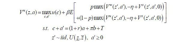
The unemployed observe their state variables at the beginning of each period and optimally choose the amount of consumption and net assets to maximize their utility from consumption given their budget constraints.7 The unemployed receive unemployment insurance benefits with probability π.8 The unemployed distribute income from net assets, unemployment benefits, and transfers from the government ( T ) to consumption and savings. The productivity of the self-employed ( z ) is independently and identically distributed ( iid ) and is assumed to follow a uniform distribution with the support of [z,z].

There exist borrowing constraints in this economy, and the maximum amount that can be borrowed is assumed to be zero following Han et al. (2017). The unemployed can become a wage worker with an exogenous probability of p by searching for jobs9 or can become self-employed without employees with a probability of one for as long as they want to be. It is assumed that the unemployed become self-employed without employees when they choose to become self-employed. For wage workers, there is no uncertainty in their labor income related to productivity because their productivity as wage workers is constant. On the other hand, for the self-employed, there is uncertainty in their business income due to the uncertainty in their productivity as the self-employed.

When the unemployed become self-employed without looking for a job, start-up costs ( η ) are incurred, and start-up costs include both monetary and non-monetary costs. For convenience of the analysis and parameterization, start-up costs are modeled as a disutility occurring during the start-up process rather than as explicit monetary costs in the budget constraints. It is assumed that there are no monetary and non-monetary costs for job search activities. If the unemployed look for a job but cannot find a job, they remain unemployed. V^w and V^s represent the value function for wage workers and for the self-employed, respectively.

2) Employed: Wage Workers

The value function for wage workers is given by

Among the employed, wage workers observe their state variables at the beginning of each period and optimally choose the amount of consumption and net assets to maximize the utility from consumption under their given budget constraints. Wage workers distribute income from labor income, net assets, and transfers from the government to consumption and savings. It is assumed that wage workers receive the minimum wage ( w ) with probability γ and the median wage ( w ) with probability 1 − γ to reflect the ratio of the minimum wage to the median wage in the model in a simple manner.

In this study, the median wage is normalized to 1 ( w = 1 ). Therefore, the minimum wage can also be interpreted as the ratio of the minimum wage to the median wage. Because γ proportion of wage workers receive the minimum wage on average, γ can be interpreted as the influence rate of the minimum wage.10 In this way, the expected earned income of wage workers becomes γw + (1 − γ)w. Wage workers experience exogenous job separation at the end of each period with a probability of χ_w and become unemployed.11 They remain wage workers with a probability of 1 − χ_w.

3) Employed: Self-employed

The value function for the self-employed is given by

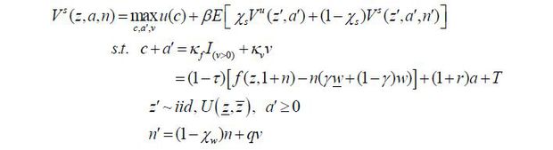
Among the employed, the self-employed observe their state variables at the beginning of each period and optimally set the amount of consumption and net assets, and the number of vacancies ( ν ) to maximize the utility from consumption under their given budget constraints. The self-employed distribute income from after-tax business income, net assets, and transfers from the government to consumption and savings.

The production function of the self-employed is given by f (z,1 + n) and it is assumed that the output varies depending on the productivity ( z ) for the self-employed and the number of employees ( n ), which change each period. The total labor input of each firm is 1 + n by adding the self-employed person and the number of employees. The price of the final product (output) is normalized to 1, which implies that the output becomes sales. The total wage cost is n(γw + (1 − γ), as the average wage paid to each employee is γw + (1 − γ)w and the number of employees equals n. Business income is defined as sales excluding wage costs, and τ proportion of business income is paid as income tax.

The number of vacancies in the current period leads to the number of employees in the next period ( n' ) with a certain probability q ( q < 1 ), an exogenous job-filling rate. Reflecting the exogenous job-separation rate of wage workers, it is assumed that the number of employees decreases by χ_w regardless of whether a business closure occurs. There is a fixed cost ( κ_f ) that must be paid for any positive number of vacancies and a variable cost ( κ_ν ) that increases according to the number of vacancies posted. I assume a fixed cost for vacancies to reflect explicitly the self-employed without employees in the model. This factor can be interpreted as explicit and implicit fixed costs in the hiring process. The self-employed experience an exogenous business closure at the end of each period with a probability of χ_s and become unemployed.12 The self-employed remain self-employed with a probability of 1 − χ_s.

Stationary Recursive Equilibrium

This model is a partial equilibrium model in which the real wage ( w ) and the real interest rate ( r ) are given exogenously. In this model, the state variables for the unemployed, wage workers, and the self-employed are given as s^u = (z,a), s^w = (z,a), s^s = (z,a,n), respectively. Correspondingly, the state space for each economic agent is defined as S^u, S^w, and S^s and the state variable for the overall economy is defined as S.

The stationary recursive equilibrium of the model is 1) a set of value functions (a value function for the unemployed ( V^u ), a value function for wage workers ( V^w ), and a value function for the self-employed ( V^s )), 2) a set of policy functions (a policy function for consumption and assets of the unemployed, a policy function for the occupational choice of the unemployed, a policy function for the consumption and assets of wage workers, and a policy function for consumption, assets, and vacancies of the self-employed), 3) transfer income from the government ( T ), and 4) a distribution function of economic agents ( μ(S) ) such that the following hold:

B. Calibration

Functional Forms

I use a standard utility function in the form of constant relative risk aversion (CRRA), which is widely used in macroeconomic studies.

The production function for the self-employed is defined as follows:

Here, n becomes zero for the self-employed without employees who perform production activities alone. On the other hand, for the self-employed with employees (employers), production activities are carried out using the number of employees including themselves. If the self-employed have higher productivity, more production is possible given the same number of employees.

Calibration of the Parameters

Parameters in this model can be divided into two groups: 1) parameters calculated outside the model or borrowed from previous studies, and 2) parameters determined inside the model in the process of matching the target statistics. Because this study quantifies the declining trend of self-employed between 2002 and 2018, the model is calibrated based on 2002. Therefore, most of the parameters and target moments used for calibration were set as of 2002, and values close to those in 2002 were used as much as possible when data were not available.

1) Parameters Calibrated Outside of the Model

The parameter for the relative risk aversion ( σ ) in the utility function is set to 2, a value widely used in macroeconomic studies. The elasticity parameter ( α ) in the production function is set to 0.85 following Atkeson and Kehoe (2005). Productivity ( z ) of the self-employed is assumed to be independently and identically distributed and the minimum value of productivity ( z ) is set to 1.492, as this value guarantees positive consumption for the self-employed. That is, consumption for the self-employed can be less than zero when the productivity of the self-employed is lower than this value.

The median wage ( w ) is normalized to be one and the minimum wage ( w ) is set to 0.334, which is the ratio of the minimum wage to the median wage in 2002. The influence rate of the minimum wage ( γ ) is set to 0.028, which is the influence rate in 2002. The exogenous job-separation rate for wage workers and the probability of business closures are set to 0.136 and 0.133, respectively, based on the exit probabilities of wage workers and self-employed in 2002 from the KLIPS data.

The real interest rate ( r ) is assumed to be 2.39% using the interest rate of the one-year Treasury Bond in 2002 (5.19%) and the CPI inflation rate in 2002 (2.8%). The annual time discount factor is set to 0.9767 to be consistent with the annual real interest rate of 2.39%. The wage replacement rate of unemployment insurance benefits is assumed to be 50% because the replacement rate has long been maintained at around 50%.13 Considering that a period in the model is one year and that the average duration of receiving unemployment benefits is approximately four months, annual unemployment benefits ( b ) are calculated and found to be 0.167 by multiplying one third of the median wage by 50%.

The probability of receiving unemployment benefits ( π ) is set to 0.046, which is the ratio of unemployment benefit recipients to the unemployed in 2002. Lastly, the effective income tax rate for the self-employed ( τ) is set to 0.135, which is the actual tax rate in 2002. The parameters calibrated outside of the model are listed in Table 1.

2) Parameters Calibrated in the Model

Six parameters are determined to match the target moments in the model. As the target moments, six labor market statistics are used. The job-finding rate for the unemployed ( p ), referring to the probability of finding jobs as wage workers, is determined to match the proportion of the employed among the labor force (87.9%) in 2002 from the EAPS. Because the population out of the labor force is excluded from the model, the proportion of employed among the total population in the model corresponds to the proportion of employed among the labor force in the data.14

The job-filling rate for the self-employed ( q ) is set to match the ratio of vacancies to the unemployed (V / U), i.e., market tightness, in the data. Although the matching function is not explicitly reflected in this study, the job-filling rate can be expressed as a function of the job-finding rate and the market tightness using a property of the constant returns to scale matching function: q = p / (V / U). Therefore, the job-filling rate can be computed using the calibrated job-finding rate and value for the market tightness (0.93) in Kim (2020).

The parameter for disutility from becoming self-employed ( η ) is determined to match the proportion of the self-employed among the employed (24.6%) in 2002 from the EAPS. The parameter for fixed costs for posting vacancies ( κ_f ) is set to match the proportion of the self-employed without employees among the employed (16.8%) in 2002 from the EAPS. On the other hand, the parameter for variable costs for posting vacancies ( κ_v ) is determined to match the proportion of employees hired by the self-employed with 1-9 employees among the employed (53.9%) in 2004 from the EAPS.15 Lastly, the maximum value for the productivity of the self-employed (z) is set to match the labor income share (58.4%) in 2002 from the National Income Accounts in Korea.

The six parameters calibrated in the model are summarized in Table 2. The annual job-finding rate and job-filling rate are set to 0.925 and 0.995, respectively. These values imply that 92.5% of the unemployed will become wage workers within one year and that 99.5% of vacant jobs will be filled within one year. The parameter for disutility from becoming self-employed is set to 3.350 and the parameters for fixed and variable costs for posting vacancies are set to 2.955 and 0.014, respectively. Considering that the annual median wage in this model is normalized to one, fixed costs for posting vacancies can be interpreted as the annual salaries of three workers. The variable cost of posting vacant jobs is determined to be relatively low. The upper limit of productivity of the self-employed is parameterized as 2.014.

Table 3 compares the target moments calculated in the model with those in the data. Although most of the target moments in the model are matched quite well, the ratio of the self-employed without employees to the employed and the share of employees hired by the self-employed with 1-9 employees cannot be matched very closely. Both target moments are related to the distribution of the size of employment. The differences appear to occur because the assumption of the probability distribution of productivity for self-employed does not accurately describe the actual case in the data.

In this model, for convenience of the analysis, the probability distribution is assumed to be a uniform distribution. However, a Pareto distribution can be used for the probability distribution of productivity, similar to Buera et al. (2011), to gain a better fit of the distribution of the size of employment. However, the focus of this study is the trend change in the number of self-employed, the sum of the number of self-employed without employees and that with employees, not the distribution of employees hired by the self-employed. Therefore, problems related to the assumption of the probability distribution may not be significant.

Table 4 shows the main statistics in the stationary recursive equilibrium. The averages of consumption and assets are 1.200 and 2.215, respectively. In the model economy, 66.3% of the total population are wage workers and 21.6% are self-employed. Because the proportion of the unemployed among the population in the model is 12.0% and the model excludes workers who are not in the labor force, the unemployment rate in the basic economy is 12.0%. In this study, workers in the agricultural sector and unpaid family workers are excluded from the model and data. Therefore, the proportion of the employed among the labor force is lower than that calculated using the entire sample. Similarly, the proportion of the unemployed in the labor force, the unemployment rate, is higher than that calculated using the entire sample.

In the model, the most important decision for the unemployed is the occupational choice between being a wage worker and self-employed. Given that the probability of being a wage worker is fixed, the more productive unemployed as self-employed are likely to become self-employed. Among the self-employed, those with relatively low productivity become self-employed without employees, and those with high productivity become self-employed with employees. On the other hand, because the cost of unemployment becomes relatively large as the amount of assets is small, the unemployed with a small amount of assets will choose self-employment when other conditions remain the same. Therefore, the unemployed with a small amount of assets can become self-employed even if their productivity is low.16

C. Quantitative Analysis

Based on the number of self-employed computed in Section 2, where the demographic structure is controlled, the number of self-employed in 2018 decreased by approximately 29.2% (0.964 million) compared to that in 2002. I quantify how much the four potential factors proposed in Section 3 can explain the change in the number of self-employed from 2002 to 2018.

Table 5 shows the changes in the parameters used in each policy experiment. In policy experiment 1 (P1), which examines the effect of the decrease in the job-separation rate for wage workers on the decrease in the self-employed, the exogenous job-separation rate changed from 13.6% in 2002 (baseline economy) to 9.8% in 2018. In policy experiment 2 (P2), which examines the effect of the increase in the income tax rate for the self-employed on the decrease in the self-employed, the income tax rate changed from 13.5% in 2002 to 14.9% in 2018.

In policy experiment 3 (P3), which examines the effect of an increase in the minimum wage on the decrease in the number of self-employed, the ratio of the minimum wage to the median wage changed from 33.4% in 2002 to 58.6% in 2018.17 Lastly, in policy experiment 4 (P4), which examines the effect of the expansion of the unemployment insurance benefits on the decrease in the number of self-employed, the ratio of unemployment insurance recipients to the unemployed changed from 4.6% in 2002 to 10.8% in 2018.

Table 6 shows the quantitative results for each policy experiment. In policy experiment 1 (P1), the number of self-employed increased by 0.24% compared to that in the baseline economy. If the job-separation rate of wage workers decreases, the inflow of wage workers to the unemployed will decrease and thus will reduce the number of unemployed who will potentially become self-employed. At the same time, however, from the viewpoint of the self-employed, a decrease in the job-separation rate for wage workers has the effect of reducing the turnover rate of their employees. A lower job separation reduces the demand for replacement hiring and the relevant vacancy costs, increasing the value of the self-employed. In the calibration of this study, the latter effect is larger than the former and the number of self-employed persons increases slightly. A notable change compared to the baseline economy is that the unemployment rate decreased by 0.023%p due to a decrease in the job separation from wage workers.

In policy experiment 2 (P2), the number of self-employed decreases by 1.00% in the base economy. An increase in the effective income tax rate reduces the after-tax business income for the self-employed, thereby lowering the value of the self-employed. The fact that an increase in the income tax rate for the self-employed leads to a decrease in the number of self-employed is consistent with the results of previous studies by Torrini (2005), Buehn and Schneider (2012), and Kang and Yoo (2018). It is noteworthy that although a 1.4%p increase in the effective income tax rate for the self-employed appears to be insufficient to explain the decline in self-employment during 2002-2018, the effect is relatively large in terms of elasticity.

The increase in the measured income tax rate in this study is likely to be underestimated for the following reasons. First, as the business income of the self-employed has been gradually reported more transparently mainly due to the expansion of credit card use (Kim and Hong, 2012), the business income of the self-employed in the past was likely underestimated. In this case, the effective income tax rate of the self-employed in the past may be overestimated, and thus the increase in the income tax rate for the period 2002-2018 may be underestimated. Second, the tax system has been changed in the direction of reducing tax exemptions and tax deductions for the self-employed since the 2000s (Kim and Hong, 2012), causing entries into self-employment to decrease and exits from self-employment to increase. Because the measured income tax rate for the self-employed is calculated only based on the self-employed who exist in the market despite the relatively large tax burdens, the measured income tax rate can be underestimated.

Given the high elasticity, the actual effect of the increase in the income tax rate on the decrease in the self-employed can be expected to be more significant considering that the increase in the income tax rate in this study can be underestimated. In other words, the actual increase in the income tax rate can be higher than that in this paper, and thus the impact of the increase in the income tax rate on the decline in the number of self-employed people may be increased considerably.

In policy experiment 3 (P3), the number of self-employed decreased by 5.11% compared to that in the baseline economy. This value corresponds to approximately 17.5% (0.169 million) of the decrease in the number of self-employed during 2002-2018 (0.964 million). In other words, the minimum wage increase explains 17.5% of the decrease in the number of self-employed during 2002-2018.18

This result for the minimum wage is consistent with the empirical results of Kang and Yoo (2018). Using linear regression estimates for panel data of OECD countries, they show that 43.5-45.2% of the decrease in the proportion of self-employed between 2000 and 2011 could be explained by the increase in the minimum wage. Although the estimated effect is less than half of that in Kang and Yoo (2018), this paper’s result supplements their empirical results in that the detailed features of the Korean labor market and the occupational choices between wage workers and self-employed are explicitly reflected in a structural model.

Intuitively, an increase in the minimum wage leads to a decrease in the number of self-employed people, especially those who have employees. In addition, the effect of the increase in the minimum wage on the self-employed without employees will be limited. Considering those who reduce their number of employees and engage in self-employment alone, the number of self-employed without employees can be expected to increase. Consistent with this prediction, in the results of this study, the number of self-employed with employees decreased significantly (-37.7%) while the number of self-employed without employees increased (16.6%).

Figure 8 shows the recent changes in the self-employed by type. A notable change since 2018 is that the number of self-employed with employees decreased significantly, whereas the number of self-employed without employees increased. The result of the experiment in this paper implies that the drastic change in the composition of the self-employed since 2018 may be closely related to the rapid increase in the minimum wage during 2018-2019.19

Finally, in policy experiment 4 (P4), the number of self-employed increases by 0.12% compared to that in the baseline economy. When the probability of receiving unemployment benefits increases, the value of the unemployed increases, which reduces the incentive to become a wage worker or self-employed. On the other hand, as the duration of unemployment increases due to the generous unemployment benefits, assets held gradually decrease. Therefore, the incentive to become self-employed can be increased because the unemployed can always become self-employed with no uncertainty. In this study, the latter effect is larger than the former given the calibration of the model. Therefore, the expansion of unemployment insurance benefits resulted in a small increase in the number of self-employed. Although the share of unemployment insurance recipients more than doubled from 4.6% to 10.8%, 89.2% of the unemployed are still excluded from receiving unemployment benefits as of 2018. For this reason, the effect of changes in the ratio of unemployment insurance recipients to the number of self-employed appears to be limited.

In sum, while the decrease in the job-separation rate for wage workers and the expansion of unemployment insurance benefits slightly increased the number of self-employed, the increase in the effective income tax rate for the self-employed and the increase in the minimum wage reduced the number of self-employed by 1.00% and 5.11%, respectively. According to the quantitative results, 17.5% (0.169 million) of the decrease in the number of self-employed people during 2002-2018 (0.964 million) can be attributed to the increase in the minimum wage.

References

, & (2005). Modeling and Measuring Organization Capital. Journal of Political Economy, 113(5), 1026-1053, https://doi.org/10.1086/431289.
, , & . (2011). Finance and Development: A Tale of Two Sectors. American Economic Review, 101, 1964-2002, https://doi.org/10.1257/aer.101.5.1964.
, & . (2018). An International Comparison of Determinants of Self-Employment Participation: Focusing on Social Policy Factors. Journal of Budget and Policy, 7(2), 129-158, in Korean, https://doi.org/10.35525/nabo.2018.7.2.006.
. (2005). Cross-country Differences in Self-employment Rates: The Role of Institutions. Labour Economics, 12(5), 661-683, https://doi.org/10.1016/j.labeco.2004.02.010.