A. Firm’s Capital Adjustment Cost

Essentially, the CAC refers to the comprehensive cost borne by firm in addition to prices formed in markets during the process of purchasing and reselling (or hiring/dismissing) production factors (capital such as equipment and labor, etc.). However, these adjustment costs do not appear in ordinary financial data. In particular, these costs can reflect the economic environment the firm faces in factor markets, the characteristics of the technology used by the firm, and the direct or indirect effects of government policies (Hamermesh and Pfann, 1996).

As Cooper and Haltiwanger (2005) point out, understanding the CAC as it pertains to investments is very important when evaluating corporate-related policies that affect investments, such as tax deductions and subsidies. However, despite the importance of investments, the CAC function for investments in macroeconomics remains a difficult problem. Moreover, because the CAC function of investments reflects various economic characteristics but is difficult to measure directly or indirectly, research on the CAC function is only conducted indirectly by studying corporate investment dynamics.

Early research on corporate investments mainly assumes the CAC to be a symmetric convex function. For example, Holt (1960) shows that the quadratic functional form of the CAC in the manufacturing industry feasibly explains firms’ hiring or layoff costs, as well as the cost of installing machinery. Cooper and Haltiwanger (2005) find that these factors as well as other external factors are reflected in the CAC. The CAC in the form of such a symmetrical quadratic function can be differentiated at all investment rates (generally net investment size/total assets), and the marginal CAC increases as the investment rate increases positively or negatively based on zero. Subsequently, in a macro model that does not take into account the heterogeneity of firms, a symmetrical convex function is mainly assumed when explaining the investment dynamics of the corporate sector. In this case, the investment level, investment dispersion, and business cycles are mainly determined by the parameters of the symmetric CAC function.

Later, in studies of firms’ heterogeneity using plant-level micro-data and corporate financial statements, the asymmetry of the CACs began to be considered in earnest. In fact, there is no reason for the marginal CAC of purchasing one unit of investment to be identical to the marginal CAC of reselling one unit. For example, if there is no secondary market for capital goods market, firms will hesitate to purchase new equipment due to uncertainty about future shocks, meaning that additional costs for capital adjustment will be incurred. The frictional cost of reselling these equipment assets is defined as irreversibility (Hamermesh and Pfann, 1996). In other words, if the CAC for reselling the equipment assets is higher than that for purchasing them due to various environmental and policy factors in the aforementioned production factors markets, it becomes difficult to sell equipment assets such as the machinery, and this irreversibility hinders firms’ active investments. Typical studies assuming an asymmetric convex function as a CAC function of investment include those by Abel and Eberly (1994) and Zhang (2005). Abel and Eberly (1994) consider the gap and irreversibility between the purchase and sale prices of capital goods as an asymmetric convex CAC, showing that the size of the investment is a non-decreasing function. In addition, Zhang (2005) shows that the irreversibility of corporate investments can generate a value premium in the stock market. In particular, he analyzes and explains the dynamics of firms in which the risk premium caused by the irreversibility of installed capital expands firms’ financial friction in the event of an economic slowdown.

On the other hand, in the manufacturing industry in the United States, several studies focus on the occurrence of lumpy investments rather than continuous investments (or the investment rate) in plant-level micro-data. In order to explain the characteristics of a period of inaction in which corporate investments do not occur, especially at the plant level, these studies report that investments do not occur continuously at all times. Instead, determination is made as to whether to invest at each time. Firms’ investment behaviors are analyzed through a discrete choice model in which the CAC function is non-convex and where irreversibility does not incur a negative investment, although there can be periods of non-investment. In relation to this, Cooper et al. (1999) argue that with regard to manufacturers, the investment is not made until equipment assets (machinery) are aged (depreciated) to a certain level, with productivity then falling below a certain level. In this model, the CAC function shows non-convexity because only fixed costs exist for a certain size of investment. In particular, this type of replacement of equipment assets often occurs when there is a positive impact on productivity, which feasibly explains how corporate investments are pro-cyclical. In the end, Cooper et al. (1999) show that this discrete investment dynamics can suitably explain the interactions among the replacement cycle of equipment assets, the cross-sectional distribution of equipment assets, and the business cycle.

B. Corporate Investments and Business Cycles

Since the beginning of modern economics, corporate investments have been among the main factors inducing business cycles because the total factor productivity shock, a major factor inducing business cycles, occurs in the production sector. If only an exogenous productivity shock occurs, ceteris paribus, a negative shock will induce a decrease in planned investments and a positive shock will induce a further expansion of planned investments. Moreover, because corporate investments are a mechanism by which to generate future cash flows, investment fluctuations can eventually widen the amplitude of business cycles. Conversely, if there is no reduction or expansion relative to a planned investment despite an exogenous productivity shock, the total production level will be determined according to the exogenous shock and the firm's planned production capacity.

Assuming that this is the case, how is the CAC function of investment related to the business cycle? As explained earlier, CACs basically refer to not only the additional costs incurred when a firm installs and employs production factors (e.g., capital, labor) but also the market environment (including the secondary market) of production factors, as well as the direct or indirect effects of government policies. Naturally, this CAC function affects a firm’s investment decisions and plays a role in expanding or reducing the amplitude of corporate investments (Hamermesh and Pfann, 1996). For example, if the CAC increases suddenly for any reason, when exogenously positive shocks occur and thus firms plan to expand their investments, they will not be able to invest as much as originally planned and the amplitude of the economic expansion will be reduced as compared to when there is no CAC. Conversely, if the CAC is lower than before due to policies that support firms, the amplitude of economic expansion may be greater. However, considering the opportunity cost for the financial resources of government policies that support firms, it cannot be inferred that the expansion of the amplitude of the business cycle necessarily maximizes social welfare.

Recent studies have shown that rational investment decision models with various CAC functions of the types described above explain various economic phenomena such as business cycles using sophisticated models with corporate financial statements or plant-level micro-data. In particular, Bloom (2009) and Bachmann and Bayer (2014) accurately show how corporate investment behaviors interact with uncertainty and affect business cycles. First, Bloom (2009) shows that a macro-uncertainty shock expands the fluctuations of gross output and employment given the temporary suspension of corporate investments and employment due to uncertainty shocks. In particular, Bloom (2009)’s model uses a mixture of convex and non-convex functions as a CAC function to assume transaction costs in the capital goods market and partial irreversibility due to resale losses in the secondary market. The parameters of the CAC function determine the period of inaction of the investment and the period in which the investment proceeds continuously.

In addition, Bachmann and Bayer (2014, expressed as BB) focus on investment dispersion of firms, showing that when the dispersion of productivity shocks for individual firms is pro-cyclical, the investment dispersion by firms is pro-cyclical. In particular, BB’s corporate model uses a discrete choice model for investment, and the CAC function is assumed to be a fixed cost. The important point here is that the investment dispersion and pro-cyclicality are strengthened as the average level of the CAC increases regardless of the distribution of individual firms’ productivity shocks and the presence of counter-cyclicality (Table 9 of BB, 2014). If the CAC rises, the investment inaction period is extended but the absolute size of the investment becomes comparatively large, meaning that the dispersion of the investment rate and the pro-cyclicality are strengthened. In this way, changes in CAC the function can affect the amplitude of business cycles.

We assume that CACs are market costs resulting from direct and indirect effects of government policies and estimate them using accounting data from financial statements. In addition, our study assesses the possibility that the CAC can significantly affect business cycles, finding correlations among changes in the CAC function, investment dispersion, and business cycles. For example, ceteris paribus, if the CAC for reselling equipment assets increases during an economic boom, the firm will make an investment smaller than the planned amount in consideration of the CAC that may be higher in the future. At the same time, firms that have suffered a negative productivity shock will reduce the scale of their restructuring of equipment assets. This means that investment dispersion is reduced compared to when the CAC for reselling assets is low, and as the efficient allocation of equipment assets is restricted, the amplitude of economic growth could be limited. Even during an economic downturn, an increase in the CAC for reselling assets causes both planned purchases and resales of equipment assets to decrease, in turn causing the investment dispersion to decrease. However, the expansion of frictional costs (CACs) for the allocation of equipment assets can cause inefficiency in the economy as a whole, which can widen the extent of an economic downturn. Changes in the CAC in relation to purchasing equipment are much clearer than those in the CAC with regard to reselling equipment assets. If the CAC for purchasing equipment fall, the economic recovery will accelerate and the extent of the economic downturn will decrease.

In fact, this interpretation is the logic of the general equilibrium model. We analyze whether the CAC function when estimated using corporate data is significantly correlated with realized investment variance and business cycles. When analyzing the relationship between the CAC function and business cycles, accurately identifying the actual exogenous shock and decomposing the effect of the CAC shock on the economy become necessary. However, because this empirical analysis model has limitations related to this type of identification, we leave this issue as a future research topic.

A. Corporate Investment and Business Cycles in Korea

This part analyzes the relationship between corporate investment behavior and business cycles through corporate data before establishing a corporate investment model. As explained earlier, to determine the shape of the CAC function, we initially check the distribution of corporate investments for every decade from 1990 to 2019. Also, in this paper, it is important to determine whether we should assume corporate investment as a continuous type of behavior or as a discrete choice in which investment inaction can also exist (Cooper et al., 1999). Given that the scope of our paper encompasses not only the manufacturing industry but also all industries, it is necessary to review in advance the possibility of the discrete choice model to analyze manufacturing businesses.

Table 1 shows the distribution of the equipment investment rates in all industries and in the manufacturing industry. First, the proportion of investment rates whose absolute value is 1% or less, indicating inactivity of investments, is 3% or less in all industries and in the manufacturing industry in all periods. These rates are much lower than the 8.1% in Cooper et al. (1999). In addition, the proportion of negative investment rates in all industries and in manufacturing exceeds 20% in all periods. This is twice as high as the rate of 10.4% in Cooper et al. (1999). Additionally, the proportions of the absolute values of positive and negative investment rates exceeding 20% are around 45% and 10%, respectively, much higher than the rates of 20% and 2% in Cooper et al. (1999). Thus, it is appropriate to use a continuous investment decision model rather than a discrete choice model. In particular, because negative investments occur frequently in the data used in our paper, we decided to use an asymmetric convex function rather than a discrete choice model, in which negative investments rarely occur.

TABLE 1

DISTRIBUTION OF REAL INVESTMENT RATES

Note: Investment rates for each year are calculated by the author using the BB model.

Source: KISData (KDI DB, 20 Jul 2020).

In addition, the correlation between investment behavior and business cycles was examined using BB’s analysis method. BB shows that investment dispersion is pro-cyclical, and Korea has a similar tendency. Figure 1 shows the distributions of investment rates in 1998, 1999, and 2019. During 1998, a severe economic slump occurred due to the Asian Financial Crisis, and 1999 was a period of recovery from this crisis. As shown in the figure, the distribution is thicker at the bottom during a sluggish economy and thicker at the top during an upturn. This occurs because the number of firms making large-scale investments (investment rates greater than 20%) increases when the economy recovers, and large-scale corporate restructuring (investment rates less than -20%) occurs when the economy is sluggish (Bachmann and Bayer, 2014).

FIGURE 1.

DISTRIBUTION OF REAL INVESTMENT RATES

Note: Investment rates for each year are calculated by the author using the BB model.

Source: KISData (KDI DB, 20 Jul 2020).

Table 2 shows the correlation between investment-rate-related variables and business cycles (GDP growth rate). It is found that the standard deviation of investment rates and GDP has a significantly positive correlation at the 1% level. Also, the correlation between the proportion of firms whose absolute value of investment rate exceeds 20% and the GDP, which affects investment dispersion, is also shown to be significantly positive.

TABLE 2

CORRELATION BETWEEN REAL GDP AND VARIABLES RELATED TO REAL INVESTMENT RATES (IRS)

Note: 1) ***, **, and * denote statistical significance at the 1%, 5%, and 10% levels, respectively, 2) Data are detrended by HP-filter.

Source: Quantiwise7; KISData.

However, recently, the correlation can be seen to weaken. This has occurred because the period of data is short (especially from 2010) and does not include events such as the Asian Financial Crisis or the Global Financial Crisis. At the same time, it is found that the positive correlation between the average investment rate and GDP has increased.

In fact, as explained above, an important investment mechanism is at work here (Bachmann and Bayer, 2014). If macroeconomic uncertainty decreases as the economy recovers, the uncertainty of firms’ productivity shocks also decreases (the pro-cyclicality of productivity shocks). Then, in anticipation of the expansion of future cash flows, firms expand their investment more than originally planned (the pro-cyclicality of investment dispersion). Thus, the additional CAC incurred by the investment will be one of the important factors determining the size of the investment. In addition, during persistent macroeconomic shocks, the CAC for positive investment is important during an economic upturn, and the CAC for negative investment is an important factor in determining the size of the investment when the economy is sluggish. However, if the CACs for production factors are large enough, the investment must be lower than the optimal investment without CACs, which will be identical even in the case of a negative shock. According to this inference, it may be reasonable to assume asymmetry of the CAC function for the investment. We will not presuppose investment irreversibility in the model. Investment irreversibility defines not only the asymmetry of the CAC but also indicates that the CAC when reselling equipment is greater than the CAC when purchasing equipment. If it is shown that the asymmetry of the CAC reflecting the direct and indirect effects of production factor markets and government policies, as explained in the previous part, has an effect on investment dispersion, the CAC will then be considered as a policy variable.

B. Corporate Investment Decision Model

In this paper, the production function of a firm is composed of individual productivity shocks ( A ), equipment assets (capital, k ), and labor ( n) according to a general model. Recent macroeconomic models set production functions by classifying intangible capital to reflect the impacts of technological innovations as well as equipment capital. However, we do not consider intangible assets separately because we focus on decision-making with regard to equipment investments, not on intangible capital. Moreover, in our paper, for simplicity of the model, it is assumed that there are no macroeconomic shocks, with only productivity shocks of individual firms following AR (1). Accordingly, a firm’s production function is expressed as

in which it is assumed that the production function follows the CRS principle (constant return to scale). Through this production function, the operating profit function is defined as follows:

where p_t denotes the product price and w_t denotes the wage. Maximization of the firm value is expressed as follows when the corporate tax rate ( τ ), equipment price ( p_i,t ), and future discount rate ( β_t ) are given.

in which i_t denotes the investment executed by the firm in period t , V_t denotes the firm value, and E_t [ • ] denotes the expectation operator. Also, the CAC function ( Φ ) is basically defined as a convex function with the form of a quadratic function; it is differentiable in the domain except at 0 given its asymmetry (Whited, 1998; Zhang, 2005).

Here, ϕ⁺ and ϕ^- are defined as parameters of the CAC function for positive (purchasing) and negative (reselling) investments, respectively. In addition, here it is not assumed that the two parameters are identical according to the assumption of asymmetry.

In the firm value maximization problem (3), the Euler equation for i_t is established as follows:

Here, the FOC of the CAC function with respect to i_t is

Equation (5) shows the effect of the CAC function on the Euler equation. First, the left side of Equation (5) shows the marginal cost for one unit of investment. The CAC parameters ϕ⁺ and ϕ^- as well as the investment rate affect the marginal cost of one unit of positive or negative investment. The right side of Equation (5) shows the future marginal return for one unit of investment, and the CAC parameters affect it in two directions; one direction is the effect of lowering future adjustment costs by investing in the present, and the other is the effect of raising future marginal costs that arise when the investment is postponed into the future. Finally, it is assumed that equipment investment and equipment assets have the following relationship:

To ensure a better understanding of the concept of the CAC function based on Equations (4) and (6), various shapes of the CAC function can be confirmed by explaining Figure 2, where (A) shows that the CAC function is both convex and symmetric. As described in the literature, this is a form that is generally assumed in a typical macroeconomic model. (B) is when the parameter of the CAC function for a negative investment is larger than the CAC for a positive investment, indicative of the assumption of investment irreversibility. Contrary to (B), (C) is a case in which the CAC function for a negative investment is lower than the CAC function for a positive investment.

FIGURE 2.

CASES OF THE CAPITAL ADJUSTMENT COST FUNCTION

As described above, this may occur when support for corporate restructuring processes such as personnel restructuring, support for the resale of used equipment assets, and deregulation are reflected. (D) refers to cases where the CAC function for a positive investment is negative. In other words, it represents a case where the total adjustment cost is lower than the theoretical equipment price in the market due to deregulation and support for equipment investment. In (E), as in (D), the CAC function for the resale of equipment is negative. Here, therefore, it is considered that used equipment assets are allocated at a price lower than the market’s theoretical price due to deregulation and efforts to support restructuring, such as the reorganization of the business. Finally, in (F), the CACs of purchasing or reselling equipment assets are all negative, meaning that they are lower than the theoretical prices in the market overall. This situation can be seen as a case where regulations on corporate investments have improved overall.

C. Empirical Data

We use the accounting data of externally audited firms (49,644 firms) for the period of 1975 to 2019 obtained from KISData and use the methods of Whited (1998), Bachmann and Bayer (2014) to convert the basic data into real variables. First, regarding the equipment asset ( k_t ) used to calculate the equipment investment rate, the sum of machinery (excluding facilities) and transportation equipment, excluding structures, is used. For the equipment investment ( i_t ), we use the sum of changes in equipment assets and accumulated depreciation according to Equation (7). Each variable is converted into a real variable using a GDP deflator, an investment deflator, and the PPI by industry (data from the BOK). In particular, the price of equipment investment by industry is converted into a real variable as follows using an equipment investment deflator and the PPI by industry (Whited, 1992):

In addition, the real investment price reflecting the tax rate for each firm is calculated as follows:

in which τ_i,t is the average effective tax rate, calculated as (Corporate Tax Expenses / Continuing Business Profit before corporate tax deduction), considering that it is impossible to use tax data held by the National Tax Service.

Also, except for the CAC function in Equation (5), a variable that cannot be inferred from the data is π_k , the marginal operating profit function. Whited (1998) estimates the first derivative for investment by defining it as follows:

in which μ denotes the mark-up for the variable cost, m_t . In other words, under the CRS assumption, the marginal operating profit is considered as the ratio of equipment assets to the margin of total sales ( y_t ). Such an estimation formula makes it easy to interpret the estimated value in the revenue function and has the advantage of estimating the markup variable at the same time. In particular, Whited (1992) estimates the parameters of CRS in the estimation equation at the same time. In this paper, μ can be interpreted as a parameter that reflects both the markup and CRS parameters (Whited, 1998). Also, y_t is the real variable of total sales, k_t is the real variable of equipment assets, and m_t is the real variable of the raw material cost.

Table 3 presents the basic statistics of 73,763 observations excluding outliers. Figure 3 shows the trends of the GDP growth rate and investment rate. As shown in Section II, the mean, standard deviation of investment rates, and the proportion of firms whose absolute values of investment rates exceed 20% appear to be pro-cyclical.

TABLE 3

STATISTICS OF BASIC DATA

Source: Quantiwise7; KISData.

FIGURE 3.

TRENDS OF GDP AND VARIABLES RELATED TO INVESTMENT RATES (IRS)

Source: Quantiwise7; KISData.

D. Empirical Methodology: GMM

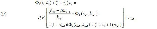
The empirical methodology used in this paper is defined as a dynamic panel GMM because the firm and year data used hear are based on the generalized method of moments (henceforth GMM) method. The specific estimation equation used as the dynamic panel GMM is derived from Equation (5) as follows:

Here, β_t is defined as the real discount rate obtained by subtracting the CPI growth rate from the one-year KTB interest rate, and δ_t is the economic depreciation rate, calculated using the formula below with the BOK’s real capital stock ( K_t ) and the real fixed capital formation ( I_t ):

The parameter vector to be estimated in Equation (9) is θ = ( μ, ϕ⁺, ϕ^-, α )' , correspondingly referring to the operating profit function, the markup versus variable cost, the marginal CAC for a positive equipment investment, the marginal CAC for a negative equipment investment, and the constant term of the CAC. In addition, because GMM mostly uses corporate financial statements, it is difficult completely to rule out endogeneity in the data. Therefore, we define the following instrument variable group ( z_t ) with reference to Whited (1992; 1998):

in which represents equipment investments to equipment assets, sales to equipment assets, raw material costs to sales, liabilities to equipment assets, operating profit to sales, and a year dummy variable, correspondingly. Given that each instrument variable must be orthogonal to the residual term ( ε_t ) defined in Equation (9), the following moment is finally derived using an instrument variable with a lag of two periods:

Here, in order to remove individual and industrial effects, an estimation formula is established by placing the difference in the residual term in a cross-relationship with the instrument variable. In addition, our GMM uses a symmetric weighting matrix for efficiency of the test statistic for the estimation according to Newey and West (1987). This is a HAC (heteroscedasticity and autocorrelation consistent covariance) matrix ( W ). Therefore, the final GMM estimation formula is expressed as follows:

In this paper, in particular according to Hansen et al. (1996) considering the finite-sample property of the GMM estimate, the weighting matrix ( W ) is modified every time from the initial value until it finally converges to find the estimate.

A. Estimation of the Capital Adjustment Cost Function

We estimate the CAC function for the period from 1978 to 2019. In particular, the total number of observations is 1,563, with only firms having more than 30 consecutive years of observations used.1

Table 4 distinguishes the CAC for a negative investment and the CAC for a positive investment. That is, after the asymmetry of the CAC function is assumed (there is no sign constraint for ϕ⁺ , ϕ^- ), the CAC function is re-estimated with the constraint that the CAC is symmetric ( ϕ⁺ = ϕ^- ). It is important to note here that asymmetry does not necessarily imply irreversibility ( ϕ⁺ < ϕ^- ).

TABLE 4

ESTIMATION OF THE CAPITAL ADJUSTMENT COST

Note: 1) ***, **, and * denote statistical significance at the 1%, 5%, and 10% levels, respectively, 2) OT is the p-value for the over-identification test, 3) LM is the p-value for ϕ⁺ = ϕ^-.

Source: Quantiwise7; KISData.

In the estimation when assuming asymmetry, ϕ⁺ and ϕ^- are estimated to be 0.13 and 1.05, respectively, and ϕ^- is estimated to be statistically significant at the 1% level. This means that the additional costs incurred during the capital adjustment process appear higher when the equipment asset is sold. This confirms that investment irreversibility as discussed in the literature may exist in Korea as well. In particular, the parameter is estimated to be 0.36 assuming symmetry of the CAC function, though the statistical significance is reduced to the 5% level. In particular, when the CAC function is constrained to be symmetric, the CAC parameter ϕ⁺ increases while ϕ^- decreases. Therefore, the symmetry constraint is likely to underestimate the CAC ( ϕ^- ) resulting from the resale of equipment assets. However, the LM test (Lagrange multiplier test) using the constraint of ϕ⁺ = ϕ^- as the null hypothesis cannot be rejected, indicating that symmetry cannot be completely excluded (Breusch and Pagan, 1980). Also, when compared to the estimates of Whited (1992; 1998), it is judged that the CAC estimated in the Korean economy is not excessive.2 In particular, the ratio of the estimates ϕ^- / ϕ⁺ = 8.1 is not an excessive gap compared to the benchmark model of Zhang (2005), ϕ^- / ϕ⁺ = 10 .3 However, the fixed cost ( α ) of the CAC function appears to be relatively high, which means that the fixed cost of maintaining equipment assets can be relatively high in the Korean economy.

In addition, in Table 4, μ , which is the markup of total sales for the variable cost, is estimated to be 1.25 at the 1%, with or without the restriction of symmetry. This value appears to be reasonable even compared to the range of parameter, [0.99, 2.26], estimated by Whited (1992; 1998). Finally, because the GMM uses more instrumental variables than the number of parameters to be estimated, over-identification tests are conducted. It appears that all null hypotheses (H0: over-identification does not exist) are rejected; accordingly, the problem of over-identification does not seem to be solved in our model, as shown in Whited (1998).

B. Capital Adjustment Cost and Business Cycles

The CAC function of the Korean economy is estimated with corporate micro-data rather than running an macroeconomic simulation as in the previous section under the assumption that the CAC function does not change from the 1970s to 2019. However, as the Korean economy has developed considerably over the past 40 years, corporate dynamics have arisen, new industries have been established, and insolvent industries have disappeared such that it is too strict to assume that the CAC function does not change such a time frame.

Moreover, as explained above, the CAC function is determined by various forms of support and by regulations affecting the equipment investment market, or the corporate restructuring support system. Therefore, it is necessary to examine changes in the CAC due to changes in government policies and labor market regulations over the past 40 years and examine how closely these are related to business cycles. To this end, if we recall Equation (5), the left side of the equation refers to the marginal cost for one unit of investment, and the right side is the expected marginal value (or expected marginal return) generated by one unit of investment. Under Equation (6), if Φ_i is higher than Φ_k due to an increase in the marginal cost, the investment will decrease. If the opposite is true, the investment will be activated. If there is asymmetry between ϕ⁺ and ϕ^- here, there are different policy implications. For example, if irreversibility ( ϕ⁺ < ϕ^- ) arises under identical conditions, the current marginal cost per unit of investment will be the same, but the future expected marginal value per unit of investment may be reduced. This eventually becomes a factor that lowers the current investment scale and can act as a mechanism affecting business cycles by reducing investment dispersion in situations where macroeconomic or individual productivity shocks are identical.4 For another example, if the CAC of equipment resales increases during an economic upturn under identical economic conditions, the firm will invest less than the planned amount of investment in consideration of uncertainty in the future. In addition, a firm that resells equipment assets in response to a current negative shock will reduce the size of the equipment to be sold if the CAC for the resale of the equipment suddenly increases. In the end, an increase in the CAC for resale of the equipment can reduce the investment dispersion and restrict the efficient allocation of equipment assets, thereby limiting the amplitude of economic growth. Looking at this in another way, if the equipment resale CAC rises even during an economic downturn, the planned purchase and resale amounts of equipment assets will both decrease. However, the expansion of frictional costs for equipment asset allocation that occurs during an economic downturn can cause inefficiency in the economy as a whole, which can widen the depth of the economic downturn. In other words, the effect of the CAC on business cycles does not simply mean the expansion or contraction of the vertical amplitude; instead, it can restrain the efficient allocation of equipment assets and negatively affect both the rising and falling periods of business cycles.

Therefore, in order to assess the changes of the CAC in the Korean economy, we estimate the CACs of firms with more than five consecutive years of data in ten-year moving windows from 1987 to 2019.5 Figure 4 shows the trends in GDP, investment-related variables, and estimates of the CAC function. For example, the estimates for 1987 are CAC functions using GMM for firms with more than five consecutive years of data from 1978 to 1987. The figure shows that the volatility of ϕ^- is greater than that of ϕ⁺ . This occurs because corporate restructuring costs such as support for corporate reorganization or regulations on manpower restructuring following the downsizing of equipment assets are more dependent on government policies. In (A) of Figure 4, the overall CAC of reselling equipment assets before the Asian Financial Crisis rises more steeply than the CAC of equipment investment, and GDP tends to decrease. During the Asian Financial Crisis, the CAC of reselling equipment assets drops sharply, as corporate restructuring was carried out smoothly as layoffs became flexible due to the pressure to undertake overall corporate restructuring and enact a non-regular-worker system in the labor market due to the crisis. However, the CAC parameters for positive equipment investment move in the opposite direction. In particular, from the early 2000s to 2016 after the financial crisis, ϕ⁺ is estimated to be larger than ϕ^- , indicating that the cost for economic growth through new equipment investments was higher than the cost of resource allocation between firms. However, because the absolute value of ϕ^- during this period was higher than ϕ⁺ , it can be inferred that even if the marginal cost of one unit of investment is high, the future marginal return is higher and the overall investment incentive increases. This can be seen in (B) and (C) of Figure 4.

FIGURE 4.

CAPITAL ADJUSTMENT COSTS AND BUSINESS CYCLES

Note: The vertical lines represent economic crises: 1998 and 2009.

Source: Quantiwise7; KISData.

(B) shows the standard deviation of the investment rate, and (C) shows the proportion of firms whose absolute value of the investment rate exceeds 20% ( | i / k |> 20% ). We can confirm that the investment dispersion is large when ϕ^- is smaller than ϕ⁺ . In addition, (D) shows the median value of the investment rates, which is also confirmed to increase when irreversibility decreases, similar to the distribution of investment rates. However, during the Global Financial Crisis, the median value of the investment rates decreases sharply. Finally, we find that the estimate of ϕ^- increases rapidly after 2017. It should also be noted that, as before the Asian Financial Crisis, the CACs for the reselling of equipment assets and supply/demand conditions worsened, and corporate restructuring costs including personnel restructuring costs increased. It is important to note that on the other hand an increase in the cost of business reorganization may represent a burden on firms during the COVID-19 crisis.

Table 5 statistically shows the correlation between the business cycles and estimators of the CACs described above. Some may point out the possibility of endogeneity in the correlation between the estimators and GDP and investment-related variables, but the parameters are estimated using corporate micro-data for ten years prior to the year of the macro variable. Therefore, it is important to note that endogeneity may not exist due to the averaging effect. It can be seen that μ , the markup of the raw material cost, and a , the constant term of the CAC function, do not have a high statistical correlation with economic variables. This stems from the fact that μ and a in the inter-temporal optimization condition (5) of the firm value maximization problem do not affect the changes in the marginal cost of investment and the expected marginal return. The important concepts here are the correlations among ϕ⁺ , ϕ^- , and the variables related to the business cycles. ϕ⁺ has a significantly positive correlation with the proportion of firms whose absolute value of the investment rate exceeds 20% and has a positive correlation, although not statistically significant, with the standard deviation of the investment rates of firms. In particular, ϕ⁺ has a significantly positive correlation with the proportion of firms with investment rates lower than -20% as compared to the proportion of firms with investment rates exceeding +20%. At the same time, ϕ⁺ appears to have a significantly negative correlation with the GDP growth rate, which means that an increase in ϕ⁺ can have a negative effect on GDP by restricting investments. However, the fact that ϕ⁺ shows a positive relationship with the proportion of firms whose absolute value of the investment rates exceeds 20% is in conflict with the existing theory, but this is due to a statistically significant relationship with large-scale negative investment. In other words, when ϕ⁺ rises, a faster decrease in ϕ^- appears to expand the resale of equipment assets. Consistent with this is that ϕ^- has significantly negative correlations with the proportion of firms whose absolute value of the investment rates exceeds 20% and the standard deviation of the investment rates. However, GDP and ϕ^- do not appear to be statistically significant. Although the degree of the reduction in the CAC of reselling equipment assets directly affects the investment decision process and thus affects investment dispersion, this is partially offset by the efficiency of the used equipment market, which can actually weaken the upward pressure on cycles. Moreover, given that output growth is not accurately decomposed with exogenous macroeconomic shocks, the impact of changes in the CACs on the economy may be mitigated.

TABLE 5

CORRELATION BETWEEN CAPITAL ADJUSTMENT COSTS AND BUSINESS CYCLES

Note: 1) ***, **, and * denote statistical significance at the 1%, 5%, and 10% levels, respectively, 2) Data are detrended by HP-filter.

Source: Quantiwise7; KISData.