
Political Economy of Immigration and Fiscal Sustainability†
Abstract
This paper introduces a politico-economic model with a welfare state and immigration. In this model, policies on taxes and immigration are determined through a plurality voting system. While many studies of fiscal implications of immigration argue that relaxing immigration policies can substitute for tax reforms in an aging economy, I show that the democratic voting procedure can dampen the effect of relaxing immigration policies as desired policy reforms are not always implemented by the winner of an election. This political economy results in three types of social welfare losses. First, the skill composition is not balanced at a socially efficient level because workers are motivated to maximize their wages. Second, older retirees implement excessive taxes to maximize the size of the welfare state. Third, the volume of immigration is lower than the optimal level given the incentive by young workers to regain political power in the future.
Keywords
Immigration, Political Economy, Fiscal Sustainability
JEL Code
E60, F22, H20, J61, D72
I. Introduction
In many developed economies, sustainability of the welfare state is an important issue. The aging of the baby-boomer generation and falling fertility rates make it more difficult to maintain welfare programs without reforms of fiscal policies. Tax reform is one option, but increasing the tax burden causes other controversies given the potential negative effects of this strategy on productivity and social welfare.
In this sense, some economists argue that relaxing immigration policies can be an effective alternative to tax reforms. According to these studies, a more liberal immigration policy for young and skilled workers can increase tax revenues and solve fiscal problems in many economies with a pay-as-you-go (PAYG) system of welfare. For example, Storesletten (2000) argues that admitting 1.6 million high-skilled immigrants aged 40-44 years old annually can replace tax reforms and resolve the fiscal problems arising in the U.S. economy as the U.S. population ages.
In most studies concentrating on the fiscal implications of immigration policies, the policy variables are assumed to be exogenous. However, during the actual immigration policy decision-making process, there are many factors, especially those that are political, that can keep desired outcomes from being implemented. For instance, young citizens of working age may worry that their wages would decrease due to competition from immigrants, causing them to vote for parties against generous immigration policies. Therefore, the extent to which the desired reforms of immigration policies can be implemented through a democratic decision-making process is important.
In this paper, I analyze political equilibria in a simple overlapping-generation model with two skill levels in labor, proportional taxes on labor income, and a welfare state in the form of simple lump-sum transfers. The native population, or the electorate, is divided into three different political parties depending on their age and skill level. The labor income tax rate, volume of immigration, and skill composition of the immigrants are then determined by the winning candidate after plurality voting. As there are three different political parties, the possibilities of strategic voting and political coalitions are also considered.
Using this model economy, I demonstrate the pattern of different preferences on fiscal and immigration policies by different cohorts. Older retirees want to maximize tax revenue per capita because they do not have labor income; hence, they prefer the Laffer rate of labor income tax and a balanced skill composition between skilled and unskilled workers to maximize production efficiency. On the other hand, the preference of younger workers depends on their skill level. Specifically, skilled workers want immigrants to be unskilled, and unskilled workers want them to be skilled. Moreover, depending on the state of the economy, young workers may not want to allow the maximum number of immigrants in, although their instantaneous utility is maximized by allowing in as many as possible. If young workers allow too many immigrants in, the probability that they lose the election in the next period increases given that the demographic composition of the electorate will be biased toward the younger generation in the next period due to the high fertility of the immigrants, which may remove the current young cohort’s opportunity to enjoy the benefit of the welfare state after they retire. Thus, older retirees want the maximum amount of immigration and the strongest welfare state as pure beneficiaries of the welfare program, while skilled young workers want zero taxes with no welfare program in most of the parameter regions. Unskilled young workers are mostly in the middle of the two groups in the sense that they do not mind taxes as much as skilled workers do. This emphasizes the role of unskilled workers as a “swing” cohort in elections.
It is also shown that the skill composition of the economy exhibits “cycling” dynamics. That is, when the skill composition is biased toward unskilled labor at the beginning of a period, unskilled workers are highly likely to sway the election, thereby approving of a high volume of skilled immigrants and balancing the skill composition. Similarly, when the skill composition leans too much toward skilled labor, skilled workers are more likely to sway the election, and the winning candidate will allow a high volume of unskilled immigrants. Since the optimal skill composition of workers is to have more skilled workers than unskilled workers in an economy with the simple Cobb-Douglas technology, the democratic procedure of plurality voting causes welfare losses due to the gap between the optimal skill composition of immigrants and the realized skill composition of immigrants, which tends to be lower than the optimal level.
I also show other factors causing welfare losses. First, the distortionary labor income tax in the model is a source of inefficiency. Because older retirees implement the Laffer rate whenever they win an election, this distortion is most severe when these retirees become the decisive political party. Second, the volume of immigration may be lower than the optimal level. Given that younger workers worry that they may not regain political power when they are older and lose their chance to obtain future social security benefits, young workers have an incentive to adjust the immigration volume to guarantee that they can win not only the election today but also those in the future.
This paper is in line with the literature on the macroeconomic implications of the political economy. Specifically, it builds on several studies on the political economy of immigration, such as Benhabib (1996), Dolmas and Huffman (2004) and Ortega (2005), and on studies of the political economy of social security systems, such as Boldrin and Rustichini (2000) and Galasso and Profeta (2002). Specifically, the main goal of this paper is to examine whether policy implications in the immigration literature1 are feasible in a positive theory setup.
This study technically follows the analyses of Ortega (2005) and Suwankiri et al. (2016). Ortega (2005) introduces a dynamic politico-economic model with immigration and skill upgrading. In his model, the voting decision of the electorate affects the skill composition of the economy, thereby influencing not only the skill complementarity but also the skill composition of the future electorate. Therefore, voters confront the tradeoff between their skill premium and their future political power. On the other hand, the work by Suwankiri et al. (2016) abstracts from skill complementarity by assuming that the production function is linear in skilled and unskilled labor. Instead, their work concentrates on a more complicated political situation in which there exists a redistributive welfare state and three political parties. The three parties, formed according to skill levels and ages, make voting decisions in a plurality voting system and, therefore, potentially vote strategically. This paper builds on the techniques introduced in both of these papers. In a state of political equilibrium, each young worker considers not only the effect of the election result on his labor income but also how it will affect his political power when he becomes older and retires.
This paper proceeds as follows. The model economy is described in section II. The political procedure of policy implementation is explained in section III. Section IV describes the political equilibria of the model. In section V, the dynamics of the model and the welfare analysis are discussed. Section VI concludes the paper.
II. Model Economy
The model builds on the dynamic overlapping generation model as in Suwankiri et al. (2016) with the application of the democracy model with strategic voting behaviors in Besley and Coate (1997; 1998). In this model, there are two generations (the young and the old) and two skill levels (skilled and unskilled). Each individual works only in the first period of his life and retires in the second and last period. The government levies proportional labor income taxes from young workers and spends lump-sum transfers via a pay-as-you-go (PAYG) system. Furthermore, the government sets the tax rate, the volume of immigration, and the skill composition of immigrants by democratic voting for each period.
In this model, each period is divided into three sub-periods. In the first sub-period, native individuals - both young and old - hold a plurality election, and the winner of the election decides on the labor income tax rate (τt), the volume of immigration (μt), and the skill composition of immigrants (σt).2 In the second sub-period, immigrants enter the economy as determined by the winning candidate. In the third and final sub-period, production, taxation, transfers, and consumption take place.
A. Preference
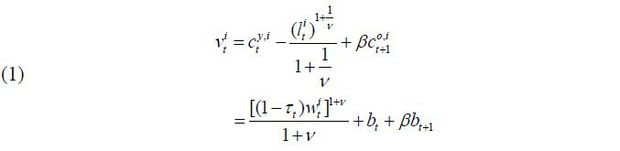
The lifetime utility function of a young worker with skill level i ∈ {s, u} is assumed to be quasi-linear in terms of consumption, as in

where  is the labor supply of skill level i ∈ {s, u}, β is the discount factor for the next period, and v is the Frisch elasticity of the labor supply.
The preference of an old retiree simply consists of the utility from today’s consumption because he does not have a future continuation value. Thus, the utility function is given by

The budget constraints of the young and the old are given by


where τt is the proportional labor income tax rate at period t, and dt and bt are savings and lump-sum transfers from the government, respectively. wt represents the wage rate.
Given that the utility function is quasi-linear in terms of consumption, the Euler equation pins down the equilibrium interest rate at a constant, i.e.,

At this rt, young workers are indifferent with respect to the amount of savings, as the marginal
benefit of savings offsets exactly the marginal cost of savings such that any amount
of savings can be an equilibrium solution. Throughout this paper, we will only consider
the case of  for all i ∈ {s, u} for simplicity. This makes old retirees simply consume the lump-sum transfer regardless
of their skill level, allowing this setup to reduce the two groups of old retirees
(skilled & unskilled) into a single group.
for all i ∈ {s, u} for simplicity. This makes old retirees simply consume the lump-sum transfer regardless
of their skill level, allowing this setup to reduce the two groups of old retirees
(skilled & unskilled) into a single group.
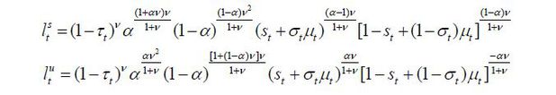
The labor supply function of a young worker with skill level i ∈ {s, u} is derived as follows:

Therefore, the indirect lifetime utility of each cohort is expressed as shown below.

B. Production Technology
This model is abstracted from capital accumulation, meaning that skilled and unskilled labor will become the only factors of production.3 The output is produced according to the Cobb-Douglas technology,

where  is the aggregate labor input of skill level i ∈ {s, u} and α is assumed to be greater than 0.5. The labor demand equations for the two skill groups
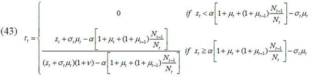
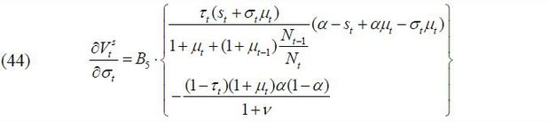
corresponding to this production function are thus expressed as shown below.
is the aggregate labor input of skill level i ∈ {s, u} and α is assumed to be greater than 0.5. The labor demand equations for the two skill groups
corresponding to this production function are thus expressed as shown below.


C. Immigration and Demographics
Before production takes place in a period, the government sets the volume and the skill composition of immigrants. For simplicity, it is assumed that only young people are allowed to immigrate; thus, all immigrants supply labor immediately upon their entrance into the economy. Then, the aggregate labor supply can be characterized by the following formulae:

in which Nt is the total size of the native young group of individuals and st ∈ [0,1] is the fraction of native-born skilled workers in the labor force in the beginning of period t. μt ∈ [0, μ] the ratio of approved immigrants to the native-born young population, thereby governing the volume of immigration.4 Finally, σt ∈ [0,1] stands for the fraction of skilled immigrants in the group of new immigrants.
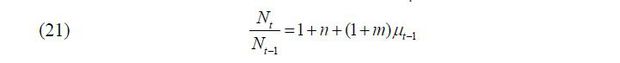
Also, there are certain additional assumptions for convenience. First, the skill levels of offspring follow the parent. Second, the offspring of immigrants are considered native, while the immigrants themselves are not.5 Then, the demographic dynamics can be described by the following equations:

where n and m represent the population growth rates for natives and migrants, respectively.6 Combining these two equations, we obtain the following law of motion for the skill composition of the natives:

Equation (3) demonstrates the role of immigration policies. For instance, σt < st implies that the fraction of skilled immigrants in the entire group of immigrants exceeds the fraction of skilled workers in the group of native young workers. Then, the fraction of skilled workers in the native young workers will increase in the next period given the assumption that the descendants succeed their parents’ skill levels. Also, if μt = 0 (no immigrants accepted), then st obviously remains the same in the next period.7 As μt → ∞ (infinitely many immigrants are approved), st+1 → σt, implying that the skill composition of the natives will converge to the skill composition of accepted immigrants as more immigration is accepted.
D. Government and the Welfare State
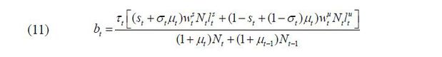
The government levies proportional labor income taxes at the rate determined by the winner of the vote. The tax revenue is transferred equally regardless of age (young and old), skill level (skilled and unskilled), and/or residence status (natives and immigrants). The government is assumed to balance the budget every period; thus, there is no government debt. The lump-sum transfer is then expressed as

in which the numerator is the total tax revenue and the denominator stands for the total population, including both natives and immigrants.
E. Equilibrium-Characterizing Equations
The general equilibrium of this economy is characterized by the following nine equations.


In this system of equations, the following variables exist:
-
• Nine endogenous variables:
 ,
,  ,
,  ,
,  , Yt,
, Yt,  ,
,  , bt, and
-
• Two state variables: μt−1 and st, and
-
• Three policy variables: τt, μt, and σt
Note that all nine endogenous variables are uniquely solvable given the state variables and the policy variables for period t. It is obvious that the decisions of output produced and labor input are purely static because there is no inter-temporal component in production, such as capital stock in a neoclassical model. However, the demographic structure of this economy is dynamic as the ratio of the native young to the native old at time t + 1 (Nt+1 / Nt) and the skill composition of the natives at time t + 1 depend on today’s decisions with regard to immigration policy (μt and σt). Therefore, the only dynamic component of this model will be the voting decision, which will be discussed in detail in section III.
The equations are further normalized by dividing by Nt , which represents the population of native young workers. The equations above can then be rewritten as follows:


where the variables with tildes are the original variables divided by Nt. For example,  is the aggregate input of skilled labor per native worker.
III. Political Decision
As discussed in Section II, the policies pertaining to the income tax rate (τt), the volume of immigration (μt), and the skill composition of immigrants (σt) are decided at the beginning of each period by the winner of plurality voting. In this section, the political decision-making process is explained in detail. This modeling of the voting process is basically identical to the application of Besley and Coate (1997) by Suwankiri et al. (2016), while there are slight differences in the electorate composition.8 In modeling the implementation procedure of the winning candidate, the idea of Markov-perfect equilibria is applied.
A. Political Decision Process
The political decision-making process of each period consists of the following three steps:
-
• Step 1: One individual is selected as a candidate in each of three political parties (the “Skilled Young,” the “Unskilled Young,” and the “Old Retirees”).
-
• Step 2: One and only one of the three candidates is elected by one single plurality voting event.9
-
• Step 3: The winning candidate chooses the set of policy variables (τt, μt, σt).
For convenience, these steps are described in reverse order in the following subsections.
1. Policy Implementation of the Winning Candidate
Once one of the three candidates is elected by plurality voting, the third and final
step of the political process is decision making by the winning candidate. The winning
candidate implements his preferred policies on taxation and immigration. As there
is no mechanism to resolve commitment problems, all voters recognize ex ante that the winning candidate will pursue his optimum after being elected, and all other
pledges are considered as 'cheap talk' under any voting equilibrium. Let the optimal
policy of the decisive candidate at time t be denoted by a triplet 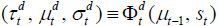 for the winning candidate’s party d ∈ {s, u, o}. Then,
  solves the following maximization problem:

where Φt+1 is the perception of today’s winning candidate of the policy variables in the next period. Obviously there can be multiple different rules of perception Φt+1 that satisfy sub-game perfection; thus, the complexity of this optimization problem depends on the multiplicity of the expectation of the policy rule of the winning candidate in the next period. If there are multiple reasonable perceptions on future policies, this period’s winning candidate must then consider multiple possibilities stemming from his decision today.
In order to refine this type of complexity and reduce the number of perceived future policy rules, this paper relies on the Markov-perfect property.10 That is, the perception function Φt+1 is assumed to be a function of the state variable for the period t + 1 only without depending on anything else, such as signals to eliminate any types of “sunspot” equilibria. With the introduction of this Markov-perfect property, the winning candidate expects that the next period’s winning candidate will make a decision according to a rule identical to those of individuals living today. Formally, the winning candidate’s problem is expressed as follows

if the winning candidate belongs to the cohort d ∈ {s, u}. Intuitively, this means that today’s winning candidate decides on policy variables with the belief that the winning candidate of the next period will decide on policy variables in exactly the same manner used by this period’s candidates, and, in any equilibrium, this belief is precisely realized.
If the winning candidate is an old retiree, his decision rule is simple given that his utility consists only of the consumption of the lump-sum payment this period. Specifically, the decision when winning the election is given by the solution of the following problem:

where bt is represented as a function of only the policy variables and the states by solving (4)~(12).
2. Voting Process
One step backward from the policy implementation procedure in section Ⅲ-A-1, now assume that one candidate is selected from each of the three political parties. The winning candidate will be determined by single plurality voting, meaning that the result of voting mainly depends on the sizes of the political parties. However, when analyzing the voting process, the possibility of strategic voting must be considered, as there are three parties. That is, if a voter believes that the candidate from his cohort has no possibility of winning the election, he may have an incentive to vote for the next-best candidate in order to prevent the worst candidate from winning the election.
Also, in this model all of the voters in the same cohort have identical preferences, implying that voters in the same political party vote identically. This setup means we must concentrate on the behavior of a representative voter instead of analyzing the complicated voting equilibrium within a cohort.
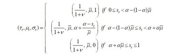
Formally, let 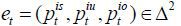 denote the voting decision of a representative voter in cohort i ∈ {s, u, o}, where
  stands for the probability that the voter in party i votes for the candidate from party j, and Δ2 is a 2-simplex. Then, voting profile
 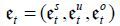 represents voting equilibrium if it solves the following problem: 11

for all i ∈ {s, u, o}, where Pj(et) is the probability that the candidate from party j wins the election given voting profile et. That is, under a state of voting equilibrium, each voter chooses for whom to vote so that the expected value of himself is maximized given the other voter’s decision and the perceived future policy of the winning candidate for the next period.
In order to reduce the possibility of multiple equilibria for a given set of state variables, I only consider the equilibria in which none of the voting decisions is a weakly dominated strategy. In addition, I assume the following tie-breaking rules for the election:
-
i) If there are two parties with the equally the largest number of votes, the candidate whose votes are from the fewest number of cohorts then becomes the winner.
-
ii) If two groups are willing to form a coalition by voting for either candidate of the two, the coalition follows the larger party of the two. If their sizes are equal, the tie is broken with equal probability.
-
iii) If the sizes of all three parties are identical, the tie is broken with equal probability.
These tie-breaking assumptions, together with the assumption that equilibria with weakly dominated strategies are excluded, guarantee that there exists a unique purestrategy voting equilibrium for each state vector of (μt−1, st). In all of these equilibria, the members of the largest (not necessarily majority) cohort always vote for the candidate from their own party regardless of the formation of a coalition; thus, a political coalition is potentially formed only by the two smallest parties.12
B. Sizes of Political Groups
Because the size of each of the political groups (groups of skilled young workers, unskilled young workers, and old retirees) is a critical component of the political decision,13 I start by looking at which group becomes the “largest” or the “majority” for all possible combinations of the state variables (μt−1, st).
The group of native skilled young workers becomes the largest group under the following conditions:
 , and
, and
Specifically, the group of skilled young workers becomes the largest if it is larger than the group of unskilled young workers and the group of native old retirees. It is clear that the first condition dominates if n + (1 + m)μt−1 > 1 while the second condition dominates otherwise.
Similarly, the group of unskilled young workers is the largest group under the following two conditions:
 , and
, and
and the first condition dominates if n + (1 + m)μt−1 > 1, with the second condition dominating otherwise.
The political party of the native old retirees becomes the largest under the following condition:

Therefore, the relative sizes of the political groups depend on the combination of the state (μt−1, st) and the parameters m (fertility rate of the immigrants) and n (fertility rate of the natives). Specifically, the relative size of the electorate groups depends on the value of n + (1 + m)μt−1, which governs the ratio between the native young and the native old. The following four cases categorize the relative size of each political group at different skill compositions st. The important fact here is that the largest group does not always win owing to the possibility that the two smaller parties form a coalition. Accordingly, this section does not describe who the winning candidate of the election is.
Case I. 
In this case, the size of the old retirees’ party is less than a third of the size
of the population of native young workers, meaning that this group can never be the
largest regardless of the skill composition of the young generation. Figure 1 displays the relative size of each political group depending on the value of st ∈ [0, 1] in this case of . The old retirees’ party constitutes the smallest group unless the skill composition
is extremely biased toward either skilled or unskilled labor, and either skilled or
unskilled workers always become the largest group.
FIGURE 1.
RELATIVE SIZES OF POLITICAL GROUPS FOR DIFFERENT SKILL COMPOSITIONS - CASE I
Note: * More than 50%.
Case II. 
This case is similar to Case I in that the old retirees never have a chance to be the largest group given that the population of the native old retirees is still less than half of the population of the native young workers.
FIGURE 2.
RELATIVE SIZES OF POLITICAL GROUPS FOR DIFFERENT SKILL COMPOSITIONS - CASE II
Note: * More than 50%.
Case III. 
This is likely to be the most interesting case. In this case, the native old population is still smaller than the population of native young workers but larger than half of it. Therefore, the group of old retirees has a chance to be the largest group if the number of skilled young workers is close enough to the number of unskilled workers. However, because the population of old retirees is still less than half of the total native population as a whole, the old retirees' group cannot constitute the majority for any value of st.
FIGURE 3.
RELATIVE SIZES OF POLITICAL GROUPS FOR DIFFERENT SKILL COMPOSITIONS - CASE III
Note: * More than 50%.
Case IV. 
In this case, the native old population exceeds that of the native young, meaning that the old retirees’ party always constitutes the majority of the electorate.
IV. Political Equilibria
As mentioned in section II, while the political decision of the policy-makers is forward-looking, the equilibrium allocation and prices are purely static in this model because there are no inter-temporal components linking different periods, such as the bond market or capital accumulation. Therefore, the equilibrium allocation can be solved analytically with only a few simplifying conditions. For instance, the equilibrium allocation is solved in a closed form if the following hold true:
-
(i) The marginal rate of substitution between consumption and leisure is multiplicative in labor input.
-
(ii) The production function is multiplicative in both types of labor (skilled and unskilled).
Therefore, a Cobb-Douglas production function and our functional form of the utility function enable the equilibrium to be solvable in closed form for a given state variable (μt−1, st) and a set of policy variables (τt, μt, σt).14 Specifically, the lump-sum transfer per capita and the wage of each type of labor are represented with respect to only (μt−1, st) and (τt, μt, σt), as follows:


Therefore, the lifetime utility of individuals in each cohort is also represented only with the state variables and the policy variables by (1) and (2).
A. Equilibria without Forward-looking
Before analyzing the equilibria of the full model, I start by demonstrating the equilibria without forward-looking behavior by individuals, which is simply equivalent to assuming β = 0. This simplified version is considered because
-
i) All equilibria associated with allocation and voting are solvable in a closed form, meaning that we can analyze all details of the equilibria, and
-
ii) More importantly, this is a good benchmark for analyzing how the forward-looking motive affects the decisions of the winning candidate and thus the voters’ choice after all.
By assuming β = 0, this model becomes abstract from the inter-temporal components, and the winning candidate’s policy decisions become a simple optimization problem of maximizing his instantaneous utility. First, we analyze the preference of each cohort with regard to policy variables, after which we examine the political equilibrium.
1. Preferences of Candidates on Policy Variables
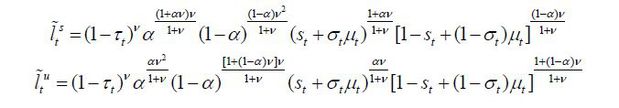
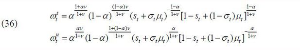
After substituting the equilibrium allocation with closed-form solutions, the utility of an individual in each cohort can be represented by the following indirect utility functions with respect to policy variables and states:

where bt and  take the form in (22)~(24) for i ∈ {s, u}. Note that the continuation value is zero for young workers as β = 0 is assumed. The ideal policies of each political party, therefore, can be analyzed
with these indirect utility functions. The following proposition displays the old
retiree’s preferred policies.
take the form in (22)~(24) for i ∈ {s, u}. Note that the continuation value is zero for young workers as β = 0 is assumed. The ideal policies of each political party, therefore, can be analyzed
with these indirect utility functions. The following proposition displays the old
retiree’s preferred policies.
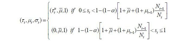
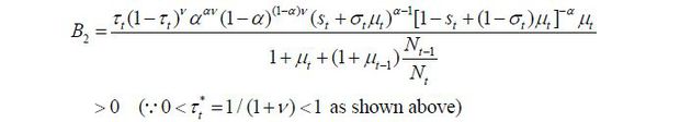
Proposition 1. If an old retiree wins the election, the implemented policy, as a result of his optimum, is characterized as follows:15
Proof. See Appendix B.1.
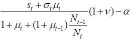
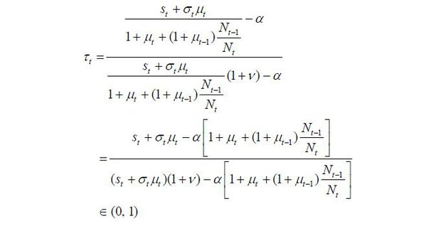
The implication of this proposition is clear: as old retirees do not have any labor endowment, they are pure beneficiaries of the welfare state. Therefore, if the candidate from the old retirees wins the election, he will choose policy variables such that the tax revenue of the government per capita is maximized. Figure 5 displays the relationship between the tax rate and the lifetime value of the old retirees. The tax rate is decided at 1 / (1 + v), which is the Laffer rate of the economy. Regarding the skill composition of immigrants (σt), the old retiree chooses σt = 1 if st is small enough and σt = 0 if st large enough, , as production and thus tax revenue is maximized when the proportion of skilled workers in the labor force equals α, the exponent in the Cobb-Douglas production function. To gain a better understanding of this implication, we assume that μ → ∞. Then, the decision of σt converges to α, which means that the old retirees want the skill composition of the economy’s workers to be consistent with the Cobb-Douglas exponent and the wage rates of skilled and unskilled labor groups to be equalized. Figure 5 shows that the value of the old retirees is maximized when σt is optimal, as in Proposition 1. Finally, the immigration volume is decided at μt = μ. This result relies on the assumption of constant-returns-to-scale technology. In other words, as long as the skill composition satisfies the optimality condition, the tax revenue is monotone increasing in the volume of immigration because the production efficiency is robust with regard to the scale of factor inputs.
The next two propositions show the optimality of the young workers with each skill level:
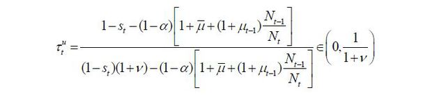
Proposition 2. If a skilled young worker wins the election, the implemented policy, as a result of his optimum, is characterized as follows:
where

Proof. See Appendix B.2.
Proposition 3. If an unskilled young worker wins the election, the implemented policy, as a result of his optimum, is characterized as follows:
where
Proof. The proof is omitted as it is symmetric to the proof of Proposition 2. Proof is provided simply by substituting st with 1 − st, σt with 1 − σt, and α with 1 − α in proposition 2.
The main implication of Propositions 2 and 3 is that young workers consider not only the lump-sum transfer but also their labor income. For example, when st is sufficiently small such that there are only a small number of skilled young workers in the economy, the wage rate of the skilled labor is so high that skilled young workers become net contributors to the welfare state, meaning that they prefer a zero tax rate. The upper panel in Figure 6 shows the utility of the skilled young workers for different tax rates and σt, the skill composition of the immigrants, when their optimal tax rate equals zero. Given a zero tax rate, the transfers also equal zero; thus, the utility of the skilled young workers depends only on their labor income. Because the wage rate for skilled labor is increasing in the input of unskilled labor due to skill complementarity, skilled workers prefer as many unskilled immigrants as possible.
The lower panel in Figure 6 displays the opposite case, i.e., where st is large enough. In this case, skilled workers now become net beneficiaries of the
welfare state because there are already excessively many skilled workers such that
the equilibrium wage for skilled labor is too small, meaning that skilled workers
prefer a strictly positive tax rate  . Nevertheless, their ideal tax rate is still smaller than the Laffer rate because
they are in any case taxpayers, while the old retirees are not. In this case, how
the skilled young workers select σt depends on two factors. First, their wage rate increases as more unskilled labor
enters the economy, as in the previous case. Second, the direction of the changes
of the lump-sum transfer depends on the pre-immigration skill composition of the economy.
Specifically, the transfer increases in σt if st is relatively small and decreases if st is large. Regardless of the size of st, however, it can be shown that the wage effect dominates the transfer effect. Thus,
skilled workers choose to approve of unskilled immigrants only.
. Nevertheless, their ideal tax rate is still smaller than the Laffer rate because
they are in any case taxpayers, while the old retirees are not. In this case, how
the skilled young workers select σt depends on two factors. First, their wage rate increases as more unskilled labor
enters the economy, as in the previous case. Second, the direction of the changes
of the lump-sum transfer depends on the pre-immigration skill composition of the economy.
Specifically, the transfer increases in σt if st is relatively small and decreases if st is large. Regardless of the size of st, however, it can be shown that the wage effect dominates the transfer effect. Thus,
skilled workers choose to approve of unskilled immigrants only.
The optimum level of unskilled young workers is symmetric to that of skilled workers, as shown in Figure 7. They set a zero tax rate when st is so large that the unskilled workers are net contributors to the welfare state, and they prefer a positive tax rate when st is small and they are net beneficiaries of the welfare state. In either case, unskilled workers prefer the maximum number of skilled immigrants.
In summary, old retirees want to maximize the government’s tax revenue by levying a high tax rate (at the Laffer rate) and balancing the skill composition of workers for efficient production. On the other hand, young workers prefer a lower (even zero) tax rate and want all immigrants to have opposite skills to maximize their disposable labor income.
2. Political Equilibria
Essentially, the result of the election depends on the relative sizes of the three political parties, as described in Section Ⅲ-B, while there is no guarantee that the largest party always wins the election given that the two smallest parties potentially form a coalition when the largest party’s preferred policy is believed to be the worst for either of the smaller groups. Therefore, not only the relative size of the electorate but also the preference of each party with regard to the preferred policies of one another will determine the result of the election.
The pattern of political equilibria depends on the relative values of the parameters.
For instance, a simple case is when  (the size of the native old population exceeds that of the native young population),
in which the candidate of the old retirees’ party always wins the election by a majority.
While equilibria can be represented in a closed form in this non-forward-looking case,
I will describe only one form of equilibrium with interesting implications rather
than considering every possible case of parameter values and states. Specifically,
the analysis concentrates on the case in which
(the size of the native old population exceeds that of the native young population),
in which the candidate of the old retirees’ party always wins the election by a majority.
While equilibria can be represented in a closed form in this non-forward-looking case,
I will describe only one form of equilibrium with interesting implications rather
than considering every possible case of parameter values and states. Specifically,
the analysis concentrates on the case in which
-
i)
-
ii) α is sufficiently large and μ is sufficiently small such that
-
iii) μt−1 is sufficiently large such that
In this case, the patterns of political equilibrium can be described by the range of st, as follows:
Case I. 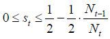
In this case, the population of native unskilled young workers constitutes the majority,
meaning that the winning candidate’s policy decision maximizes the lifetime value
for the unskilled young. Because st is so small in this case that the unskilled young workers become net beneficiaries
of the welfare state, the choice of the winner’s policy variables is 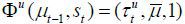 , where
  is defined as in Proposition 3. Whether a political coalition arises is immaterial
as it cannot take the majority.
is defined as in Proposition 3. Whether a political coalition arises is immaterial
as it cannot take the majority.
Case II. 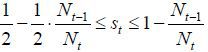
In this case, the party of the unskilled young workers is still the largest but does
not secure a majority. However, the smallest parties (the skilled young workers and
the old retirees) do not have any incentive to form a coalition because they perceive
that the policies of the other party are the worst. For the old retirees, the preferred
policy of the skilled young includes a zero tax rate, which is the worst for the old
retirees as it leads to a zero welfare state. For the skilled young workers, the policies
of σt for both the unskilled young workers and the old retirees are equally the worst because
both prefer σt = 1, while the old retirees even prefer a higher tax rate. Therefore, for both the
old retirees and the skilled young workers, it is the next-best choice to let the
unskilled workers win the election, thereby forgoing the possibility of a political
coalition. As a result, the unskilled young workers' party wins the election and the
winner implements 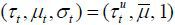 according to Proposition 3.
Case III. 
In this case, the population of old retirees is the largest, the unskilled workers are the second, and the skilled workers form the smallest group. Therefore, it is important as to whether the skilled and unskilled workers have an incentive to form a coalition with each other. It is clear that the skilled workers have an incentive to vote strategically for the unskilled candidate. The preferred tax rate of the unskilled workers is τu ∈ (0, 1 / (1 + v)), which is advantageous for the skilled workers as it levies fewer taxes than the old retirees would levy. Both the old retirees and the unskilled workers prefer the maximum number of skilled immigrants. Therefore, the skilled workers are willing to vote for the political party of the unskilled workers. Because the population of unskilled workers exceeds that of skilled workers, the coalition is formed such that the unskilled candidate represents the overall coalition. Therefore, the unskilled workers win the election.16 The policy implementation becomes (τt, μt, σt) = (τu, μ, 1) according to Proposition 3.
Case IV. 
In this case, the population size is still the order of the old, the unskilled, and the skilled. The only difference from the previous case is that now the unskilled workers are net contributors and thus prefer zero taxes, as also wanted by the skilled workers. Therefore, the coalition is formed so that the unskilled party wins the election, and the policy of (τt, μt, σt) = (0, μ, 1) is implemented according to Proposition 3.
Case V. 
In this case, the old retirees are the largest group, the skilled are the second-largest, and the unskilled are the smallest in size. Also, because both skilled and unskilled workers are net contributors to the welfare state, both groups prefer a zero tax rate; thus, the old retirees equally dislike both young candidates and want neither to win. The skilled workers obviously prefer the unskilled workers’ policy profile to that of the old retirees. Therefore, the important problem is whether the unskilled prefer the skilled workers’ ideal policy to the old retirees’. If the unskilled workers prefer skilled workers, the skilled candidate would then represent the coalition. Otherwise, the unskilled workers would have no reason to vote for the skilled workers, meaning that the skilled workers strategically vote for the unskilled workers' candidate, and the unskilled candidate will represent the coalition.
For the unskilled workers, the preferred policies of the other two parties have the following trade-offs: Though the skilled workers’ preferred policy, denoted by (τt, μt, σt) = (0, μ, 0), is preferable because it levies zero taxes, it will allow many unskilled immigrants in and make the competition in the unskilled labor market tighter. Though the old retirees’ preferred policy, denoted by (τt, μt, σt) = (1 / (1 + v), μ, 0), is beneficial because it will allow in a maximum number of skilled immigrants, it levies high taxes on labor income. Therefore, the problem is whether the unskilled workers can bear the high tax rate (at the Laffer rate) preferred by the old retirees in order to allow as many skilled immigrants to enter as possible. Formally, this trade-off is characterized by the threshold tax rate, denoted by 𝜏̃(μt−1, st) and determined implicitly by solving for the following equation:
Vu(μt−1, st ; τt = 𝜏̃, μt = μt, σt = 1) = Vu(μt−1, st ; τt = 0, μt = μt, σt = 0), where the left-hand side is the utility of the unskilled workers when the tax rate is at 𝜏̃ and the maximum number of skilled immigrants are approved, and the right-hand side is the utility of the unskilled workers when the skilled young workers’ candidate wins the election.17 In other words, 𝜏̃ is the maximum tax rate that the unskilled young workers can bear in return for approving the maximum number of skilled immigrants. If 𝜏̃ < 1 / (1 + v), then the tax rate to be levied by the old retirees is excessively burdensome to the unskilled, meaning that the unskilled will strategically vote for the skilled workers’ party. Otherwise, if 𝜏̃ ≥ 1 / (1 + v), the unskilled workers then prefer the old retirees’ policy at least as much as the skilled workers’; thus, a coalition is formed such that the unskilled candidate represents the overall coalition and wins the election.
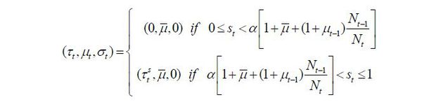
As a result, the skilled young workers' candidate wins the election with the support of the unskilled party if 𝜏̃ < 1 / (1 + v), which implements (τt, μt, σt) = (0, μ, 0) according to Proposition 2. If 𝜏̃ ≥ 1 / (1 + v), then the unskilled workers win the election with the support of the skilled workers and the policy implementation is (τt, μt, σt) = (0, μ, 1) via Proposition 3.
Case VI. 
In this case, the order of electorate size is as follows: skilled, the old retirees, and then the unskilled. As in the previous case, the old retirees do not have an incentive for strategic voting because all of the young workers prefer a zero tax rate. Therefore, the problem is whether the unskilled are willing to vote strategically for the old candidate or not, and this decision depends on the level of the unskilled workers’ threshold tax rate 𝜏̃. If 𝜏̃ ≤ 1 / (1 + v), he unskilled do not participate in the coalition with the old retirees and the skilled party wins; thus , the policy implementation will be (τt, μt, σt) = (0, μ, 0) according to Proposition 2. If 𝜏̃ > 1 / (1 + v), then the old retirees win the election with the support of the unskilled workers, and the resulting policy implementation is given by (τt, μt, σt) = (1 / 1 + v), μ, 1) according to Proposition 1.
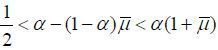
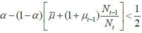
Case VII. α − (1 − α)μ < st ≤ α + αμ
In this case, the order of the electorate size is identical to that in the previous
case (the skilled, the old retirees, and then the unskilled). The difference is that
now st is so large that the old retirees prefer a “balanced” skill composition of immigrants
at  instead of allowing skilled immigrants only. This makes the unskilled workers less
favorable to the old retirees, thereby decreasing the threshold tax rate for strategic
voting. Formally, the new threshold tax, denoted by
instead of allowing skilled immigrants only. This makes the unskilled workers less
favorable to the old retirees, thereby decreasing the threshold tax rate for strategic
voting. Formally, the new threshold tax, denoted by  , is determined implicitly by the following equation:

If  , the unskilled do not participate in the coalition with the old retirees and the
skilled party wins; thus, the policy implementation will be (τt, μt, σt) = (0, μ, 0) according to Proposition 2.
, the unskilled do not participate in the coalition with the old retirees and the
skilled party wins; thus, the policy implementation will be (τt, μt, σt) = (0, μ, 0) according to Proposition 2.  , then the old retirees win the election with the support of the unskilled workers;
thus,
, then the old retirees win the election with the support of the unskilled workers;
thus, 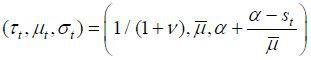 is implemented via Proposition 1.
Case VIII. 
In this case, the electorate size is identical to that in the previous case (the skilled, the old retirees, and then the unskilled). However, now st is so high that the old retirees want to implement σt = 0. Therefore, neither the old retirees nor the unskilled workers have an incentive to support each other. As a result, no coalition is formed and the skilled candidate wins the election as the largest party. The policy of (τt, μt, σt) = (0, μ, 0) is implemented according to Proposition 2.
Case IX. 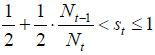
In this case, the skilled young workers’ party constitutes the majority of the electorate. The skilled young candidate wins the election and implements (τt, μt, σt) = (0, μ, 0) via Proposition 2.
The nine cases above describe the patterns of political equilibria depending on the skill composition and the age composition of the economy. In short, a highly unbalanced skill composition makes the larger skill group more likely win the election, and the old retirees are likely to win when the young-to-old ratio is small enough and the skill composition of the young voters is relatively balanced. The forward-looking case will be shown to exhibit a similar pattern of equilibria in the next section.
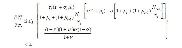
B. Equilibria with Forward-Looking Characteristics
In this section, the young workers now care not only the instantaneous utility but also for their own future value (alternatively, β > 0). This results in a trade-off for the young workers. For example, for an unskilled young worker, it is still advantageous to approve of many skilled immigrants because the skill complementarity will increase his wage during this period, as discussed in the previous section, without forward-looking behavior. However, forward-looking behavior now imposes a drawback on this strategy. If too many skilled young immigrants enter the economy during this period, the descendants of those immigrants will be native skilled young workers in the next period (meaning that they have the right to vote in the next period as members of the skilled young party). Therefore, it is highly likely that the skilled young workers’ party, which is most hostile to the welfare state, will win the election during the next period. This will deprive the present unskilled workers of the future welfare state after they retire. The unskilled young workers of this period can predict this and thus may choose to approve of only a small number of skilled workers so that the skilled young workers will not constitute a majority in the next period.
Formally, if a young candidate with skill level d wins the election, his policy rule is determined by the following optimization problem:
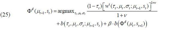
subject to

An old retiree’s decision when he wins is identical to that in the previous section when β = 0 because his utility does not depend on the future.
Due to the complexity of this model, I rely on a numerical solution for this forward-looking case. Essentially, the solution numerically searches for the functional form of Φd (μt−1, st) which solves the functional equation (25).18 In other words, the solution describes what the winning candidate’s optimal choice of the policy profile is given the state vector.
Figure 8 displays which cohort actually wins the election given the state vector (skill composition of the electorate on the horizontal axis and the young-to-old ratio of the electorate on the vertical axis). First, the red line divides the state space into three regions according to in which the largest party is. For instance, regions (a) and (d) are where the unskilled workers’ party forms the largest group, regions (b), (e), and (g) are where the skilled workers’ party is the largest, and the old retirees’ party is the largest in (c), (f), and (h). The blue line further divides the regions according to which group becomes the winner and how this group wins. The following details can explain this:
-
• In regions (a), (b), and (c), either one of the groups constitutes the majority (more than 50%) of the electorate. Therefore, the political party with the majority wins the election.
-
• In region (d), the unskilled party is the largest. It wins the election because the two smaller parties (the skilled and the old retirees) are expected to implement a policy profile which is the worst to the other; thus, no coalition is organized.
-
• In region (e), the old retirees’ party wins while the skilled workers group is the largest because the unskilled young workers prefer the old retirees’ policy profile to that of the skilled. In other words, the unskilled workers can bear the high tax rates that the old retirees are expected to levy as the old retirees will approve of many skilled immigrants and increase the wages of the unskilled labor.
-
• In region (f), the unskilled workers’ party wins the election though the old retirees are the largest because the skilled workers strategically vote for the unskilled candidate to keep the old retirees from winning the election.
-
• In region (g), the skilled workers’ party wins the election as the largest party. The other two parties do not form a coalition.
-
• In region (h), the skilled workers’ party wins the election by forming a coalition with the unskilled. The old retirees’ party is the largest but fails to win because their preferred tax rate (the Laffer rate) is excessively burdensome to the unskilled workers.
Therefore, a political coalition is formed in (e), (f), and (h), while the smaller parties let the largest to win without the formation of a coalition in (d) and (g).
Figure 9 shows how the winning party and the equilibrium volume of immigration differ according to the skill composition of the voters for a fixed young-to-old ratio of the electorate. While the old retirees always approve of the maximum number of immigrants, young workers can choose a value smaller than the maximum for certain values of st. Note that this occurs solely due to forward-looking behavior, as the desired immigration volume is always the maximum level without the forwardlooking component, as shown in Propositions 1~3.
Figures 10~12 describe why unskilled workers prefer μt < μ in some states and μt = μ in others. In Figure 10, the current state is given by point A. Path (i) shows how the economy will move to a new state in the next period if the winning candidate decides to approve of the maximum number of immigrants. As the diagram demonstrates, allowing the maximum number of skilled immigrants will make skilled workers the majority group in the next period, thereby removing the possibility of receiving transfers after they retire. To prevent this, an alternative option for the unskilled workers is to approve of a slightly smaller number of immigrants instead (path ii), which will guarantee that today’s unskilled young workers will win the election again in the next period (and thus receive the maximum lump-sum transfer), though it will reduce today’s labor income of the unskilled workers relative to path (i). Figure 11 shows an example in which it is too costly to reduce the immigration volume so as to win in the next period if the economy is currently at point B. In this case, the unskilled workers will abandon the possibility of winning in the next period and attempt to maximize today’s utility by allowing the maximum number of immigrants, which explains why the immigration volume increases to its maximum at around s = 0.6 in Figure 9.
Finally, Figure 12 depicts a case in which it is not feasible for unskilled workers to regain political power in the next period by adjusting the immigration volume. If the skill composition is sufficiently biased toward unskilled labor, unskilled workers cannot make the economy move toward a state in which old retirees will win the election in the next period even if the maximum number of skilled immigrants is accepted. In this case, the unskilled workers’ optimal choice is simply to approve of the maximum number of skilled immigrants to maximize the instantaneous piece of their utility.
V. Dynamics and Social Welfare
In this section, the dynamics of the key macroeconomic variables and their implications are analyzed. According to the analysis of political equilibria shown in the previous section, the skill composition of the economy is the key component which determines who wins the election and how the policies are implemented. Moreover, based on the results, it is expected that the skill composition exhibits cyclical movement; if the skill level of the young natives (i.e., young voters) is biased toward unskilled labor, the skill composition will move toward skilled labor in the next period because the unskilled workers’ party is highly likely to win the election and approve of the maximum number of skilled immigrants, whose descendants will be skilled workers in the next period. Similarly, if the proportion of skilled workers is very large, the skill composition will move toward unskilled labor in the next period by the same logic.
This cyclical behavior of the skill composition leads to welfare loss in the economy. Because the production function of this model is the Cobb-Douglas aggregation of skilled and unskilled labor with exponent α for skilled labor, the socially optimal skill composition is obviously such that α is the proportion of skilled labor and 1 − α is that of unskilled labor. In this sense, the skill composition selected by the old retirees is socially optimal, while the young workers’ ideal decision may be suboptimal.
In this model, immigration per se does not cause any inefficiency due to the constant-returns-to-scale technology. In other words, it is socially optimal to approve of as many immigrants as possible as long as the post-immigration skill composition becomes more balanced toward α. Therefore, the welfare loss in this economy is three-fold. First, the skill composition is not always balanced because young workers prefer maximal skill complementarity to maximize their own wages. Second, the proportional labor income tax is distortionary. Third, young workers may not choose to allow the maximum number of immigrants in to regain their political power in the following period.
A. Welfare Loss due to a Skill Imbalance
In order to check whether the skill composition exhibits a suboptimal path, the dynamics of the skill composition is examined in this section. Figure 13 displays the dynamics of the post-immigration skill composition of workers when α = 0.8 , and the initial skill composition equals 0.5. As surmised in the previous paragraphs, the skill composition fluctuates over time. For instance, skilled workers win the election at t = 2 , decreasing the proportion of skilled workers by allowing the maximum number of unskilled immigrants. This causes, at t = 3 , the unskilled workers to win the election and pushes the skill composition upward. The old retirees win the election at t = 4 because the unskilled workers adjust the immigration volume at t = 3 so that they can be the decisive party again when they retire. Given that the old retirees want the skill composition to be balanced at α, the skill composition of immigrants is adjusted such that the skill composition of workers is precisely at α after the immigrants enter the economy. This causes the skilled workers to win the election at t = 5 , and this pattern is repeated later on.
It is notable that the value of st always stays below α. Because α is assumed to be larger than 0.5 for the skill premium, the skilled workers’ party is likely to win the election when st is close to α. Therefore, the welfare loss from the skill imbalance is mainly caused by the skilled workers in this model. This skill imbalance not only causes a welfare loss but also dampens the effect of immigration in sustaining the welfare state. Given that the welfare state is most efficiently financed when st = α, ∀t , the gap between α and st caused by the skilled workers’ ideal policy deteriorates the inefficiency of the welfare state.
Furthermore, the fluctuation of the skill composition converges to the same pattern of cycles regardless of the initial skill composition. Figure 14 shows how different initial skill compositions in the end exhibit the same cyclical behavior. The skill composition converges to identical cycles because the value of st is pulled into α whenever the old retirees win an election. In other words, whenever the old retirees’ party wins an election, the economy is absorbed into the state of st = α in the next period.
Figure 15 displays the dynamics of wage rates for skilled and unskilled labor, respectively. It is clear that the skilled workers implement a policy profile to maximize their own wage (e.g., t =1) and that unskilled workers maximize their own wage (e.g., t = 2 ). The wage rates are equalized at t t = 3, t = 6, and t = 9 , denoting the period when the old retirees win an election. The implication is simple; as discussed above, the Cobb-Douglas exponent and the actual skill composition will be equalized by the old retirees. At the same time, the income share of the skilled workers is always α according to the property of the Cobb-Douglas technology. Therefore, the wage rates for both skills are equalized when the old retirees win an election and implement the “skill-balancing” immigration policy.
B. Welfare Loss by Distortionary Taxation
It is obvious that the labor income tax in this model distorts the labor supply of both skills. This type of welfare loss is mainly caused by the old retirees because they prefer the Laffer rate to maximize the welfare state. As proved in Proposition 2 and Proposition 3, the tax distortion is either zero or is smaller than that caused by the old retirees if any cohort of the young workers becomes the decisive party. Therefore, the principal contributors of the welfare loss by taxes are the opposite of those in the case of the skill imbalance: the old retirees are the main contributor, and the skilled workers’ preferred tax policy is the least distortionary in terms of taxation.19
Figure 16 shows the implementation of the tax rate over time. It is straightforward to observe
that the old retirees levy  at the Laffer rate, while the skilled workers levy zero taxes. The unskilled young
workers implement a small non-zero tax rate when they win, as proved in Proposition
3.
at the Laffer rate, while the skilled workers levy zero taxes. The unskilled young
workers implement a small non-zero tax rate when they win, as proved in Proposition
3.
C. Welfare Loss by an Immigration Volume Adjustment
In this model, the only reason for the immigration volume to be smaller than μ is the young workers’ motive to regain political power after they retire, as discussed in section Ⅵ-B. Figure 17 shows the implemented volume of immigration over time. Note that the volume does not reach its maximum at t = 5 and t = 7 , both of which are the periods when the unskilled workers win an election. However, in this numerical example, the gap between μ and the implemented μt is very small; moreover, such a value of μt that is smaller than μ is still very large (nearly 1, which means that an identical number of immigrants equal to that of the existing native young workers enters the economy).
VI. Concluding Remarks
This paper analyzes a politico-economic model of immigration and the welfare state to demonstrate the patterns of the political equilibria and the theoretical implications of sustainability of the welfare state and efficiency of the economy. In this two-period overlapping- generation model, the size of the welfare state, the volume of immigration, and the skill composition of immigrants are determined by the winner of a plurality voting system for each period. Because there are more than two political parties, the possibilities of strategic voting and consequent political coalitions among small political parties are also considered.
In the political processes, there are two key conflicts among the cohorts: the old vs. the young (maximizing the welfare state vs. low taxes) and skilled workers vs. unskilled workers (more unskilled immigrants vs. more skilled immigrants). In equilibrium, the skill composition of immigrants is biased toward unskilled labor relative to a socially efficient level because, at the socially efficient level of skill composition, the skilled workers' party is more likely to win the election. Due to this inefficiency, the effect of the immigration policy on the sustainability of the welfare state is weaker than expected when considering the literature.
Different sources of welfare loss are also analyzed. Not only does the imbalance of the skill composition contribute to the welfare loss but so also do distortionary taxation and the suboptimal volume of immigration. Specifically, the ruling of the old retirees causes maximal tax distortion, as these retirees want to maximize tax revenues by the government. If a young cohort becomes the ruling party, the volume of immigration can be determined at a level lower than the optimal level due to the young workers’ incentive to regain political power in the future.
Finally, this study does not consider the possibility that the winning candidate’s implementation of immigration policy is not feasible due to, for example, a lack of foreign-born workers who want to migrate to the host country. Also, another interesting case not studied here is one in which there are masses of refugees potentially entering several countries, and the refugees’ country choice depends on the policy of each country as well as the economic state, such as the skill composition, aggregate productivity, and demographic structure.
Appendices
APPENDIX
A. Full Equilibrium Solution of Allocation and Prices
If the production function is a typical Cobb-Douglas function in skilled and unskilled labor, the equilibrium can be represented by closed-form expressions.20 In other words, all instances of equilibrium allocation and prices are represented in closed-form functions of the policy variables (the labor-income tax rate, the volume of immigration, and the skill composition of immigrants), state variables (μt−1 and st), and the parameters. For a Cobb-Douglas production function, the equilibrium is characterized by the following nine equations:


with nine unknowns 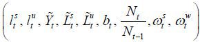 , each of which is defined as in section 2.
Plugging (29) and (30) into (26) and (27), respectively, leads to

Because at this point the equations are expressed in terms of variables for labor
input only, this becomes a system of two equations and two unknowns ( and
and  ) when substituting
  and
and  with the (31) and (32) solutions. After some algebra, labor input per skilled and
unskilled worker is represented only by the following policy variables and parameters:
with the (31) and (32) solutions. After some algebra, labor input per skilled and
unskilled worker is represented only by the following policy variables and parameters:
By plugging these back into (31) and (32), we obtain the following closed-form expressions
of total skilled and unskilled labor divided by the native young population ( and
and  , respectively):
By plugging these further back into (28), the output per native young worker  is also represented in a closed form, as follows:

Consequently the amount of the lump-sum transfer (bt) is represented in the function of policy variables and states according to the results above.

Finally, the wage rates of skilled and unskilled labor are calculated as shown below.
B. Proofs
B.1. Proof of Proposition 1
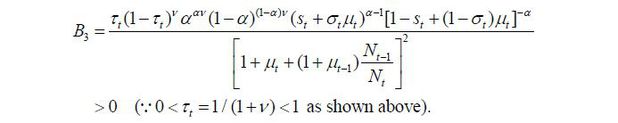
The old retirees’ objective function at time t is simply the lump-sum transfer per capita:

Thus, we can differentiate it by each of τt, μt, and σt using (35).
First, the derivative with respect to the tax rate is


where

Obviously  at either τt = 1 / (1 + v) or τt = 1. However τt = 1 implies no lump-sum payment by (35) and thus zero utility for the old retirees,
meaning that τt = 1 / (1 + v) is the optimal tax rate when the old retiree group wins the election.
at either τt = 1 / (1 + v) or τt = 1. However τt = 1 implies no lump-sum payment by (35) and thus zero utility for the old retirees,
meaning that τt = 1 / (1 + v) is the optimal tax rate when the old retiree group wins the election.
Second, the derivative of  with respect to the skill composition of immigrants is as follows:

where
Note that  for any σt ∈ (0,1) if st > α + αμt, and
  for any σt ∈ (0,1) if st < α + αμt − μt. Therefore, the optimal choice of the skill composition of immigrants when the old
retirees' party wins an election is expressed as shown below.
for any σt ∈ (0,1) if st < α + αμt − μt. Therefore, the optimal choice of the skill composition of immigrants when the old
retirees' party wins an election is expressed as shown below.

Finally, the derivative of with respect to the volume of immigration is
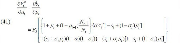
where
There can be three cases according to the optimal decision for σt.
Case I. st ∈ (α + αμt, 1]
In this case, σt = 0 as shown in (40). After substitution, (41) is rewritten as follows:
Therefore, because  for any value of μt, it is optimal to choose μt = μ.
Case II. st ∈ [0, α + αμt − μt]
In this case, σt = 1 as shown in (40). After substitution, (41) is rewritten as follows:
Therefore, because for any value of μt, it is optimal to choose μt = μ
Case III. st ∈ [α, + αμt − μt, α + αμt]
In this case, 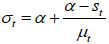 as shown in (40). After reorganization, (41) is rewritten as follows:
After substituting  , the first term equals zero, and the entire expression is simplified into the following
form:
, the first term equals zero, and the entire expression is simplified into the following
form:

Therefore the optimal choice is μt = μ.
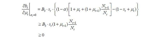
In conclusion, given that  is strictly positive, the optimal choice of the old retiree is to choose μt = μ regardless of the state of the economy, which ends the proof.
B.2. Proof of Proposition 2
The skilled young worker’s objective function at time t consists of two terms: the utility from the lump-sum transfer and the utility from the labor income net of the disutility of working:

First, the derivative of  with respect to the tax rate is expressed as follows:

Because  by (36). Plugging (36) and (38) into this expression yields
where

Therefore, the optimal tax rate for a skilled young worker depends on the state of the economy (st, μt−1), and the following two cases are possible:
Case I. 
In this case we can observe the following two consequences:
-
i)
 , and
, and
-
ii)
 is either is either a positive number or a negative number smaller in terms of the
absolute value compared to
is either is either a positive number or a negative number smaller in terms of the
absolute value compared to 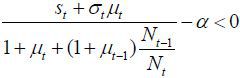 .
.
These two observations guarantee that  . Therefore, the optimal tax rate for a skilled young worker in this case is given
by τt = 0.
. Therefore, the optimal tax rate for a skilled young worker in this case is given
by τt = 0.
Case II. 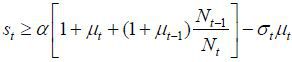
In this case, we have an interior solution at
Therefore, these two cases show that the optimal decision of τt for the skilled young worker is given by
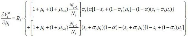
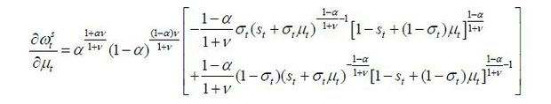
The derivative of  with respect to the skill composition of immigrants is

Plugging (36) and (39) leads to
where

Again, the optimal decision of σt can be separated into two cases, as in (43).
Case I. 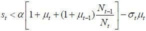
In this case, the optimal τt is zero according to (43). After plugging τt = 0 into (44), obviously  , implying that the optimal σt equals zero.
Case II. 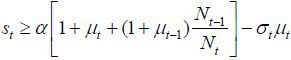
This case is equivalent to 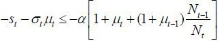 . Plugging this inequality into (44),
Because  for both cases, the optimal decision of σt is always zero for the skilled young worker.
Finally, the derivative of the skilled young worker’s objective function with respect to the volume of immigration is expressed as follows:

As it was already shown that σt = 0 in the optimum state, we can use (42) to derive the following:

and there can be two cases depending on the value of st :
Case I. 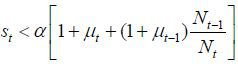
In this case, τt = 0 as shown above; therefore, bt = 0 and thus  .
.
Case II. 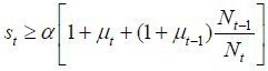
In this case:
Therefore,  is non-negative in either case. Now, the derivative of the wage rate is written in
detail as follows:
is non-negative in either case. Now, the derivative of the wage rate is written in
detail as follows:
Substituting σt = 0, it is readily apparent that  , thereby implying that
  . Therefore, the optimal choice of the volume of immigration for the skilled young
worker is μ.
. Therefore, the optimal choice of the volume of immigration for the skilled young
worker is μ.
At this point, we return to the intervals of st in (43). Because now we know that μt = μ and σt = 0 in optimality, we can substitute μt and σt with μ and 0, respectively, ending the proof.
C. Political Coalition and Equilibria
In this section, I discuss the details of the assumption of the determination process of political equilibria as discussed in section Ⅲ-A-2. As in the model, there are three political parties, and all of the individuals in one party have identical preferences. Throughout this section, let A, B, and C denote the three political parties in the order of their population sizes and #(A), #(B), and #(C) denote the relative sizes of the three parties, respectively. The sizes are normalized such that #(A) + #(B) + #(C) = 1 such that the measure of the size of the overall electorate equals 1.21 We assume that all parties have at least one member; formally, this is #(X) > 0 for all X ∈ {A, B, C}.
First, it will be proved that the largest party’s members always vote for their own party regardless of whether they constitute the majority or not. It is obvious that #(A) > 0.5, which is a trivial case. Hence, we assume that it does not exceed 50%. Then, Lemma 4 follows:
Lemma 4. A member of A votes only for A in any political equilibrium.
This implies that the members of the largest political party do not vote strategically for a candidate from another party in any of the equilibria after repeatedly eliminating weakly dominating strategies. The proof is shown below.
Proof. It is obvious that the members of A prefer A’s policy profile most. Accordingly, we can assume, without a loss of generality, that the members of A prefer B to C. Then, it is obvious that C is weakly dominated by the other two strategies. Therefore, we assume that there is a state of equilibrium in which A’s members vote for B. Then, the following possible cases exist:
Case I. B’s members vote for B, and C’s members vote for C.
In this case, for C’s members, voting for B gives a weakly smaller payoff than voting for A because if A’s members deviate to voting for A, then A wins the election.
Case II. B’s members vote for C, and C’s members vote for B.
Similar to Case I.
Case III. B’s members vote for B, and C’s members vote for B.
Then, for the members of A, voting for A and B results in an identical payoff because C wins after all.
Case IV. B’s members vote for C, and C’s members vote for C.
Similar to Case III.
Therefore, in any of the cases above, voting for B is at least weakly dominated by voting for A, which contradicts the assumption that voting for B occurs in equilibrium and ends the proof.
Therefore, it is clear that the members of the largest cohort always vote for the candidate of their own cohort. Together with this lemma, the following assumptions refine the political equilibrium so that there is a unique form of pure-strategy equilibrium per state.
-
(i) Weakly dominated strategies are repeatedly eliminated.
-
(ii) If there are two parties with the equally the largest number of votes, the candidate whose votes are from the least number of cohorts then becomes the winner.
-
(iii) Voters strategically vote for the candidate of another cohort only if it is strictly preferred to not doing so.
-
(iv) Suppose there are two parties. If all members of both parties prefer to form a coalition with each other, the candidate of the larger party out of the two becomes the candidate of the overall coalition. If the sizes of the two parties are identical, the candidate is determined by equal probability.
-
(v) Any remaining possibility of ties is broken with equal probability.
These assumptions, together with Lemma 4, imply the following results of the election.
Case I. #(A) ≥ 0.5
This is the simplest case to solve, where A’s candidate wins the election by a majority. Note that #(A) = 0.5 also guarantees A’s victory due to assumption (ii) above.
Case II. 0.5 #(A) > #(B) ≥ #(C)
This is the most interesting case. Because A does not take the majority, it is important as to whether B and C form a political coalition or not, which depends on the preference of B’s and C’s members. The following exclusive and exhaustive cases are possible:
-
• Case II-1. B’s members at least weakly prefer A to C, and C’s members at least weakly prefer A to B.
-
In this case, neither B nor C wants a coalition because they perceive the other party's ideal policy to be the worst. Therefore, A wins the election by receiving the largest number of votes.
-
• Case II-2. B’s members at least weakly prefer A to C, and C’s members strongly prefer B to A.
-
In this case, while B’s members do not have any incentive to vote for C strategically, C’s members have an incentive to vote for B’s candidate. Therefore, B’s candidate represents the political coalition by B and C and wins the election in the equilibrium.
-
• Case II-3. B’s members strongly prefer C to A, and C’s members at least weakly prefer A to B.
-
In this case, C’s candidate represents the coalition by B and C wins the election via the same logic presented in Case II-2. Note that C wins the election despite the fact that it is the smallest cohort in the electorate.
-
• Case II-4. B’s members strongly prefer C to A, and C’s members strongly prefer B to A.
-
In this case, both of the two smaller parties want to form a coalition. If #(B) > #(C) , then the candidate of B represents the entire coalition according to assumption (iv) and wins the election. If #(B) = #(C), then the candidate of the coalition is determined by a coin toss, and the resulting candidate wins the election.
Case III. #(A) = #(B) > #(C)
In this case, C serves as the swing cohort. If C’s members strongly prefer A to B, then A wins the election by forming a coalition with C. If’ C’s members strongly prefer B to A, B wins the election similarly. If C’s members are indifferent, then they do not vote strategically, and either A or B then wins the election with equal probability (a coin toss).
Case IV. #(A) = #(B) = #(C)
In this case, each party wins the election with a probability of 1/3.
Notes
This paper is written based on Chapter 1 of Hur, 2016, Essays on Fiscal Policy, University of California, Los Angeles.
As explained above, many studies report that relaxing immigration policies can reduce fiscal problems in developed economies. Among others, see Auerbach and Oreopoulos (1999) and Storesletten (2000).
An alternative setup for this is to assume that capital stock per capita is fixed and that immigrants bring the same amount of capital stock when they are approved to immigrate.
The volume of immigration has a finite upper bound because otherwise the choice of µt can be infinity in a number of political equilibria, as the production function is a constant-return-to-scale function. In an economy with DRS technology, µt has a finite value even without an exogenous upper bound. In this DRS case, however, the state of the economy depends not only on the relative population size of the voters but also the absolute number of young workers, thereby increasing the dimension of the state vector by one.
In other words, immigrants cannot vote for their lifetimes, while their descendants are legal voters.
In many developed countries, it is consistently observed in census data that the fertility rate is higher for immigrants than for natives, implying m > n. One recent example is the report of U.S. Census Bureau by Monte and Ellis (2014).
In other words, immigration is the only method of changing the aggregate skill composition in this model, and there is no skill acquisition or loss. For studies focusing on the transition of the aggregate skill level or task composition through immigration, readers can refer to Hunt and Gauthier-Loiselle (2010) and Peri (2012), among others.
For example, Suwankiri et al. (2016) simplifies the political equilibria in two aspects. First, they assume that only the smallest party out of the three can choose to vote strategically, thereby eliminating the possibility that the smallest party wins the election. Second, they assume that immigrants have the right to vote when they become old. This simplifies the equilibrium because the young-to-old ratio in the electorate is consistent with that of the whole pre-immigration population. Both simplifications are relaxed in this paper; the smallest party can win an election if the members of the second-largest party have an incentive to vote strategically and the smallest party’s members do not have incentive to vote for the second-largest party. Also, immigrants do not have the right to vote for their lifetimes in this paper.
In other words, there is no second voting such as, for example, the run-off primary in the U.S. presidential election.
The Markov-perfection property in this paper is taken directly from Suwankiri et al. (2016), which builds on the Markov-perfection setup used in previous works on short-term government and political economy, such as Krusell and Rios-Rull (1996), Grossman and Helpman (1998), and Hassler et al. (2003).
It is implicitly assumed that there is no additional cost for the electorate to participate in voting, and only equilibria in which none of the voters abstains are considered.
As emphasized before, note that the size of the electorate is not the only component, as whether a coalition is formed or not depends not only on the relative size of the two smallest groups but also on their policy profile preferences with regard to the others parties.
Obviously, some of the ranges of 𝑠t can be an empty set if μ is large enough. For instance, if μ is larger than α/(1 − α), the optimal σt always equals because the first and the third intervals become empty sets.
I do not consider whether the unskilled workers have incentive to vote strategically for the skilled candidate because the unskilled workers’ party is a larger group than that of the skilled workers and the skilled group does have an incentive to vote for the unskilled candidate. In this case, regardless whether the unskilled party’s secondbest choice is the skilled workers' candidate or not, the coalition is formed such that the unskilled workers' candidate represents the overall coalition according to the equilibrium refinement procedure introduced in Section III-A-2. Obviously, the case in which the skilled party wins the election by forming a coalition with the unskilled workers can be a form of Nash equilibrium if the unskilled workers have incentive to do so.
For the solution to (25), a grid for the state vector (𝜇, 𝑠') is constructed and fixed points are found by iteration. Though the solution is checked for several initial points for robustness, uniqueness is not mathematically proved in this study. It is hoped that this issue will be solved in future studies.
Although skilled workers potentially prefer a non-zero tax rate, as proved in Proposition
2, it is mostly not realized because these workers prefer a non-zero rate only if
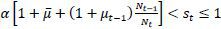 , which is an empty set for most reasonable values of
  , μ, and α. For instance, the interval becomes empty for the following conservative choice of
parameters: α = 0.8, μ = 0,
, μ, and α. For instance, the interval becomes empty for the following conservative choice of
parameters: α = 0.8, μ = 0,  .
.
References
, & . (1999). Analyzing the Fiscal Impact of US Immigration. The American Economic Review, 89(2), 176-180, https://doi.org/10.1257/aer.89.2.176.
. (1996). On the political economy of immigration. European Economic Review, 40(9), 1737-1743, https://doi.org/10.1016/0014-2921(95)00122-0.
, & . (1997). An economic model of representative democracy. The Quarterly Journal of Economics, 112(1), 85-114, https://doi.org/10.1162/003355397555136.
, & . (2000). Political equilibria with social security. Review of Economic Dynamics, 3(1), 41-78, https://doi.org/10.1006/redy.1999.0072.
, & (2004). On the political economy of immigration and income redistribution. International Economic Review, 45(4), 1129-1168, https://doi.org/10.1111/j.0020-6598.2004.00300.x.
, & . (2002). The political economy of social security: a survey. European Journal of Political Economy, 18(1), 1-29, https://doi.org/10.1016/S0176-2680(01)00066-0.
, & . (1998). Intergenerational redistribution with shortlived governments. The Economic Journal, 108(450), 1299-1329, https://doi.org/10.1111/1468-0297.00344.
, et al. (2003). The survival of the welfare state. American Economic Review, 93(1), 87-112, https://doi.org/10.1257/000282803321455179.
, & . (1996). Vested interests in a positive theory of stagnation and growth. The Review of Economic Studies, 63(2), 301-329, https://doi.org/10.2307/2297854.
. (2005). Immigration quotas and skill upgrading. Journal of Public Economics, 89(9-10), 1841-1863, https://doi.org/10.1016/j.jpubeco.2004.06.012.
. (2012). The effect of immigration on productivity: Evidence from US states. Review of Economics and Statistics, 94(1), 348-358, https://doi.org/10.1162/REST_a_00137.
. (2000). Sustaining Fiscal Policy through Immigration. Journal of Political Economy, 108(2), 300-323, https://doi.org/10.1086/262120.
, , & . (2016). The welfare State and migration: a dynamic analysis of political coalitions. Research in Economics, 70(1), 122-142, https://doi.org/10.1016/j.rie.2015.07.001.