
Korea’s Inflation Expectations with regard to the Phillips Curve and Implications of the COVID-19 Crisis†
Abstract
This paper estimates the expectation-augmented Phillips curve, which explains inflation dynamics, in Korea. The phenomenon of low inflation in Korea has been going on for quite some time, in particular since 2012. During the Covid-19 crisis, due to low inflation expectations the operation of monetary policy was limited as the base rate approached the zero lower bound. The main objective of this paper is to estimate where and how tightly inflation expectations are anchored. It was found that long-term inflation expectations fell to around 1%, falling short of the inflation target, and that inflation expectations are strongly anchored to long-term expectations, which implies that the low inflation phenomenon is likely to extend into the future. The results also imply that even if inflation fluctuates due to temporary disturbances, it may converge to a level below the inflation target. The slight rebound of long-term expectations during the Covid-19 crisis suggests that the aggressive monetary policy may have contributed to improving economic agents’ beliefs about the commitment of monetary authorities to inflation stability. This may also help long-term expectations gradually to approach the inflation target.
Keywords
Inflation Expectations, Phillips Curve, Monetary Policy
JEL Code
E31, E42, E52
I. Introduction
The continuing phenomenon of low inflation remains ongoing in Korea. Figure 1 shows the inflation targets and the actual inflation rates. Prior to 2011, inflation sometimes fell outside the range of the target temporally, but for most of the period inflation it was in line with the targeted forecasts. In contrast, since 2012 actual inflation has been below the inflation target for most of the period. Short-term disturbances, such as international oil price hikes, a good harvest, bird flu, and footand-mouth disease, may play major roles in headline inflation fluctuations. However, core inflation, which excludes food and energy, has also been gradually declining below the target since 2012.
FIGURE 1.
THE COVID-19 CRISIS IN KOREA
Note: Shading represents the inflation target.
Source: Statistics Korea.
As the phenomenon of low inflation has continued, economic agents may have lowered their inflation expectations, which have limited the operation of monetary policy. If the economy is subdued and inflation falls, the monetary authority in Korea lowers real interest rates (nominal interest rates minus inflation expectations) by cutting the key short-term nominal rate, the base rate. Given that nominal interest rates are bounded by zero, real interest rates cannot be sufficiently lowered when inflation expectations are low.
When the Covid-19 crisis occurred, the Bank of Korea cut its base rate to a level close to the lower bound. That is, due to low inflation expectations, the Bank of Korea could not sufficiently adjust real interest rates. As the base rate approached the lower bound, the Bank of Korea employed unconventional monetary policy measures, such as purchasing government bonds, whose effectiveness is uncertain and debatable. Recognizing the importance of the stable expectations, the Bank of Korea revised its “General Principles of Monetary Policy Operation” in December 2020. According to the new general principles, the Bank of Korea is supposed to consider anchoring of inflation expectations in addition to overall inflation and growth outlooks, the associated uncertainties and risks, and financial stability conditions when it assesses the path of convergence of inflation.
Stable inflation expectations themselves matter with regard to the stability of actual inflation. If expectations are well anchored, actual inflation is ensured to converge to the target even if it temporally deviates. The sustained low inflation in Korea, however, suggests that expectations may not have been well anchored. If expectations are tightly anchored to a level that differs from the target, it becomes difficult to expect inflation to converge to the target in the foreseeable future. With this motivation, the main objective of this paper is to estimate where and how tightly inflation expectations are anchored.
Several previous studies have investigated possible decreases in the slope of the Phillips curve, inflation’s responsiveness to economic fluctuations. Ball and Mazumder (2011; 2019) found that US expectations of the Phillips curve were strongly backward-looking in the past, but became more strongly linked to the Fed’s inflation target recently. Based on this evidence, they concluded that inflation remained stable in the 2000s, not because the slope of the Phillips curve had decreased but because inflation expectations had been strongly anchored. Matheson and Stavrev (2013), the IMF (2013), and Blanchard, Cerutti, and Summers (2015) also analyzed the Phillips curve for the United States or for 21 countries. They also found that inflation expectations for the US were strongly anchored to long-term expectations recently.
This paper also studies variations in inflation expectations in the Phillips curve by applying the Kalman-filter model used in Matheson and Stavrev (2013), the IMF (2013), and Blanchard, Cerutti, and Summers (2015). An obvious difference is that this paper analyzes the Korean economy, which was not considered in the previous literature. A more critical departure is that this paper directly estimates long-term inflation expectations, in contrast to existing literature. For long-term expectations, Ball and Mazumder (2019) used the Fed’s target level, while Matheson and Stavrev (2013), the IMF (2013), and Blanchard, Cerutti, and Summers (2015) used survey results. Considering the upward bias of survey results in Korea, using survey results as a proxy for long-term inflation expectations in the Phillips curve is limited. This paper found that while inflation expectations in Korea also show recent strongly anchored to long-term expectations, the anchored level appears to be substantially different from the target.
There have also been studies of the low inflation phenomenon in Korea from a structural point of view. Lee (2014) and Jung (2019) investigated the low inflation phenomenon, the risk of deflation, and implications for monetary policy. Lee (2014) and Cho (2018) compared Japan’s economic structure and macro-policies with Korea’s. Japan’s monetary policy was critically examined, and policy implications were derived to prevent deflation in Korea, whose current economic structure is similar to that of Japan’s in the past. Jung (2019) and Cho (2020) discussed structural issues in the Korean monetary policy management system. Although this paper does not formally analyze Korea’s monetary policy, it suggests related policy implications.
This paper is organized as follows. Section II discusses the survey results on inflation expectations. Section III presents the model and data. Section IV shows the results and implications, and Section V concludes the paper.
II. Discussion of Survey Results
Inflation expectations are unobservable. This section discusses the survey results on inflation expectations. The Bank of Korea surveys the public and experts on inflation expectations. Surveys of the general public are released monthly, and surveys of experts are released through a quarterly monetary policy report. Inflation expectations refer to the rate of headline inflation over the following year. Figure 2 shows that expectations of the general public are higher than those of experts.
FIGURE 2.
SURVEY RESULTS ON INFLATION EXPECTATIONS (ONE-YEAR-AHEAD)
Source: Bank of Korea, Consensus Economics.
Consensus Economics examines inflation expectations with experts. This survey concentrates on headline inflation, categorized into short-term (one year ahead) and long-term (five years ahead) periods. The survey results of experts by the Bank of Korea and Consensus Economics are very similar because the survey groups who take the two surveys are similar. In this paper, experts’ expectations will be discussed based on the survey conducted by Consensus Economics because it has a longer time series.
First, this paper examines whether the survey results have a statistical bias. As a simple benchmark, I also examine inflation of the current period as the forecast for one-year-ahead inflation. In the first column of Table 1, when current inflation is used as a forecast for inflation expectations, an upward bias of 0.1%p is found. This can be understood as reflecting the trend in which inflation rates have declined by 0.1%p per year. Inflation expectations for the general public has an upward bias of 1.0%p compared to actual inflation, meaning that the upward bias is much greater than the expectations when using current actual inflation. The fact that there is upward bias in inflation expectations over a long period of time means that there is a limitation to predicting future inflation trends with survey results on inflation expectations of the general public. Experts’ inflation expectations also showed an upward bias of 0.3%p from actual inflation rates. The bias of expert inflation expectations was smaller than that of the general public, but it was also found to be greater compared to the simple use of current actual inflation. This suggests that it is difficult even for expert groups to forecast inflation trends.
Table 1 shows the size of the average error of inflation expectations against the actual future inflation, as measured using the root mean squared error (RMSE). If current-period inflation is used as the inflation forecast, the RMSE is about 1.2%p, as presented in Table 1. Inflation expectations of the general public have an RMSE of 1.5%p, which is larger than the forecast error of the current actual inflation. This also means that the inflation expectations of the general public are less useful than the current inflation value in explaining short-term inflation fluctuations.
The bias reveals a more pronounced difference since 2012, when inflation began to fall persistently below the target. Table 1 shows that the upward bias of the inflation expectations for the general public is larger and that the RMSE is also higher. The bias of experts’ inflation expectations was also relatively large. For reference, the bias of expert inflation expectations before 2012 was −0.2%p.
TABLE 1
ONE-YEAR-AHEAD INFLATION EXPECTATIONS AND ACTUAL INFLATION
Note: One-year-ahead inflation expectations  are formed at period t−4 and compared with actual inflation πt at period t. Bias denotes the averages of forecast errors
  and the RMSE (root mean squared error) is determined using the eqution
Source: Bank of Korea, Consensus Economics, Statistics Korea.
How can we determine why the bias of inflation expectations for the general public is high and the forecasting error is large, and what are the main factors affecting the formation of inflation expectations? Previous studies such as those by Lee (2012), Choi (2012), Lee and Choi (2015), and Nam and Go (2018) explained that the backward-looking factor in the formation of inflation expectations is important. The Bank of Korea’s survey of the general public includes inflation perception as well as inflation expectations. Inflation perception comes from the results of a survey on headline inflation over the previous year. Figure 3 shows the inflation expectations of the general public, inflation perception results, and actual inflation. First, we find that there is a considerable gap between the general public’s perception of inflation and actual inflation. Second, inflation expectations are strongly correlated with inflation perception, indicating that the formation of inflation expectations is backward-looking. Nam and Go (2018) reported that these features were also found in other major economies.
FIGURE 3.
INFLATION EXPECTATIONS, INFLATION PERCEPTION, AND ACTUAL INFLATION
Source: Bank of Korea, Statistics Korea.
With regard to long-term inflation expectations, Consensus Economics surveys experts on five-year-ahead inflation expectations. Figure 4 compares the survey results on short- and long-term inflation expectations. While long-term expectations tend to fluctuate around the inflation target, short-term expectations have consistently fell short of long-term expectations, meaning that the survey respondents thought that inflation would gradually converge to the inflation target in the future. Just as there was upward bias in short-term expectations, however, long-term expectations also show some upward bias. In contrast to the experts’ long-term expectations, actual inflation has been below 2% for most of the period since the second half of 2012.
FIGURE 4.
SURVEY RESULTS ON LONG-TERM AND SHORT-TERM INFLATION EXPECTATIONS
Source: Consensus Economics.
The discussion covering the survey results on inflation expectations can be summarized as follows. First, the inflation expectations of survey results tended to be backward-looking. Second, the short- and long-term expectations did not correspond to the low inflation phenomenon that has appeared since 2012. Therefore, it is highly likely that the results of the inflation expectations survey did not sufficiently reflect information on the future inflation trend.
III. The Model and Data
This section explains the method used to estimate inflation expectations as reflected in the time series of actual inflation. After setting the Phillips curve model, we explain how we measure where and how strongly inflation expectations are anchored by a Kalman-filter model.
A. Phillips Curve Model
The Phillips curve represents how prices are determined. The specific form may vary from study to study, but in this paper, inflations are expressed as inflation expectations, demand-side pressure, and supply-side pressure. This form of the Phillips curve is also supported by a theoretical model. For example, Clarida, Galí, and Gertler (1999) derived the following Phillips curve in the dynamic stochastic general equilibrium model:

where ŷt denotes the GDP gap. Given that inflation expectations in Clarida, Galí, and Gertler (1999) are purely forward-looking, past inflation is not included on the right side of the Phillips curve. Woodford (2003), Christiano, Eichenbaum, and Evans (2005), however, explained that in the model in which producers index prices to past inflation, past inflation may be included in the Phillips curve.
Inflation expectations can be expressed in various forms. The simplest form is the
adaptive expectations form, i.e.,  If economic agents believe that inflation will converge to a certain level, they
may not adjust inflation expectations to one-to-one for short-term fluctuations in
inflation. For example, Ball and Mazumder (2019) set inflation expectations as a weighted average of long-term inflation expectations
and past short-term inflation. Economic agents’ long-term inflation expectations may
also change over time.
If economic agents believe that inflation will converge to a certain level, they
may not adjust inflation expectations to one-to-one for short-term fluctuations in
inflation. For example, Ball and Mazumder (2019) set inflation expectations as a weighted average of long-term inflation expectations
and past short-term inflation. Economic agents’ long-term inflation expectations may
also change over time.
Demand pressure is usually estimated by the GDP gap. In many previous studies, demand pressure is measured by the unemployment rate gap. However, in Korea, the unemployment rate is of limited utility when used to explain economic fluctuations.1
According to Chun (2020), factors of global inflation can help to predict Korea’s inflation. Global factors can include both global demand pressure and global supply pressure, and can be expressed as global inflation. This paper measures global factors using import price inflation.
Based on the above discussion, the Phillips curve can be set as follows:

where πt denotes inflation,  inflation expectations, ŷt the GDP gap,
  import price inflation, and et other factors including short-term supply factors.
Following Matheson and Stavrev (2013), the IMF (2013), and Blanchard, Cerutti, and Summers (2015), inflation expectations are set as the weighted average of longterm inflation expectations and past short-term inflation,

where πt denotes long-term inflation expectations and  is past inflation. θt represents the stability of inflation expectations or the degree of anchoring to
long-term expectations. As θt is high, inflation is less affected by short-term factors. Finally, the Phillips
curve is set in the following form.
is past inflation. θt represents the stability of inflation expectations or the degree of anchoring to
long-term expectations. As θt is high, inflation is less affected by short-term factors. Finally, the Phillips
curve is set in the following form.

This paper sets constraints on the coefficients following Matheson and Stavrev (2013), the IMF (2013), and Blanchard, Cerutti, and Summers (2015). Because inflation expectations are the weighted average of long-term expectations and past short-term inflation, 0 ≤ θt ≤ 1. As the widening of the GDP gap and the rise in import price inflation push up domestic inflation, κt ≥ 0 and γt ≥ 0. Long-term inflation expectations are unconstrained.
B. Kalman-filter model
This paper uses the Kalman-filter model, details of which can be found in Hamilton (1994), among others. To reflect the constraints, we consider the following transformation:

For all βt ∈ (−∞, ∞), the constraints are satisfied. The inverse transformation can be written as

Let  denote the predetermined exogenous variables and let

Observation equations in the Kalman-filter model are πt = h(βt, xt)+et, where the error term is independent and identically distributed and follows a normal distribution, et ~ N(0, R), State equations are

where the error term is independent and identically distributed and follows a normal distribution, vt ~ N(0, Q). The covariance matrix Q is a diagonal matrix. The state equations imply that the state variables βt follow a random walk pattern.
In a linear Kalman-filter model, the observation equation is expressed as πt = Htβt + et. In contrast, h(βt, xt) is non-linear in βt and hence the model in this paper is a non-linear Kalman-filter model. In this paper, not only is the nonlinear transformation applied to reflect the constraints, but there are also cross terms between state variables in the observation equations. To analyze the non-linear Kalman-filter model, this paper follows Simon and Chia (2002), Simon (2010), and Matheson and Stavrev (2013), among others. The key procedure is to replace Ht with the gradient of h(βt, xt) with respect to βt.

Taking partial derivative, I obtain

The forward recursion of the Kalman filter includes
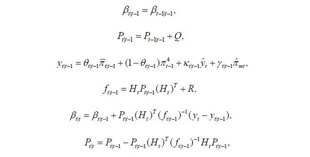
where for any variable zt, zt1|t2 denotes the estimate for zt of period t1 based on information up to and including period t2. Given the parameters (R, Q), I calculate the likelihood using the Kalman filter and then obtain the maximum likelihood estimates for (R, Q).
By Kalman filtering, I obtain βt|t, which is the estimate with the information up to period t. The main focus of this paper is not the short-term forecasting of πt but is instead the trends of πt and θt per se. It is more useful to obtain estimates for πt and θt with all available information. To obtain βt|T I apply backward recursion to the Kalman smoothing,

The backward recursion of the mean squared error matrix follows:

C. Data Description
The sample period is from the first quarter in 2000 to the fourth quarter in 2020. Inflation is measured as the logarithm difference of quarterly seasonally adjusted consumer-price indices. Because the seasonally adjusted consumer price is not officially released, Census X-13 ARIMA-SEATS values are used. I multiplied the difference by 400 in each case to convert the rates into the annual percentage change. The past short-term inflation is the year-over-year logarithm difference relative to the consumer price of the previous period. This corresponds to the average quarterly inflation over the four quarters. I multiplied the difference by 100. This specification followed Matheson and Stavrev (2013), the IMF (2013), and Blanchard, Cerutti, and Summers (2015).
The GDP gap is the actual GDP(Yt) and the potential GDP(Yt ). That is, ŷt = (ln Yt − ln Yt ) × 100. The potential GDP is unobservable and thus needs to be estimated. This paper uses the method of Hodrick and Prescott (1997), henceforth referred to as the HP filter. Estimates of the potential GDP with quadratic time trend are also examined. Figure 5 shows the GDP gap estimates by the two methods. The overall trends of the two series are very similar, but there are some differences in the breadth of the economic fluctuations. The methods using the structural VAR model in Blanchard and Quah (1989) is widely used in the literature. Blanchard and Quah (1989) used data on the unemployment rate and GDP. In Korea, the unemployment rate is limited if used to reflect short-term economic fluctuations. Because the HP filter and the quadratic time trend model mechanically decompose the time series into trends and short-term fluctuations, the accuracy of the potential GDP estimation is debatable. In future research in this area, more rigorous estimates of the GDP gap could be used to improve the results of this paper. Therefore, when interpreting the results of this study, it is necessary to focus more on the estimation of inflation expectations rather than on the coefficient of the GDP gap.
Import price inflation is defined as the logarithm difference of seasonally adjusted import prices in Korean won relative to consumer prices in accordance with Matheson and Stavrev (2013), the IMF (2013), Blanchard, Cerutti, and Summers (2015). Import price inflation is also converted into an annual rate. The deviation from the mean is calculated by subtracting the mean value of the sample period from the time series. In a regression analysis, the mean value of the time series is often treated as a constant term. In this analysis, however, because a constant term may affect the level of inflation expectations, the mean value of the time series is subtracted.
IV. Results and Implications
A. Linear Regressions
Before performing the Kalman filter analysis, I undertake a linear regression analysis. This model is usually used to identify short-term inflation fluctuations. We consider the linear regression analysis below.

This regression model can be interpreted as meaning that the form of inflation expectations is expressed as follows:

The long-term expectations are πt = c and the degree of anchoring is θt = (1 − ρ). The other coefficients are also assumed to be invariant over time.
Table 2 shows the results of regression analysis with the sample from the first quarter of
2000 to the fourth quarter of 2020. The dependent variable is quarterly headline inflation
in the annual rate. The coefficient of is estimated to be 0.519, which means that there is considerable inertia affecting
inflation. Inflation also had a statistically significant response to the demand pressure,
i.e., the GDP gap. Inflation was analyzed and found to increase by 0.056%p when import
price inflation rises by 1%p, and this was found to be significant at the 1% level.
TABLE 2
LINEAR REGRESSION ESTIMATIONS
Note: 1) Numbers in parenthesis are Newey-West standard errors, 2) ***, **, and * indicate significance at the 1, 5, and 10 percent levels, respectively.
The implied degree of anchoring to long-term inflation expectations is 1 − 0.519 = 0.481. The implied long-term inflation expectations are 1.032 / (1 − 0.519) = 2.15%, which is less than the average of the inflation target levels.
Table 2 also shows the result of the same analysis on core inflation. The coefficient of
is estimated to be 0.706, indicating that the inertia of core inflation exceeded
that of headline inflation. There was no significant difference between headline and
core inflation outcomes with regard to the response to the GDP gap. On the other hand,
for core inflation, the regression coefficient for import price inflation was small
and statistically insignificant; while changes in energy prices have a strong influence
on import price inflation, they are excluded from the basket of core inflation.
The implied degree of anchoring to long-term inflation expectations is 1 − 0.706 = 0.294. The implied long-term inflation expectations are 0.579 / (1 − 0.706) = 1.97%, similar to the estimate using headline inflation.
The linear regression model above can be interpreted as meaning that the state variables
are assumed to be constant over time. This assumption may be improper considering
that there was a declining trend of the inflation rate in Korea. To examine this possibility,
rolling regressions were performed. The same linear regression model was analyzed
with the data for 40 quarters (ten years) from period t − 39 to period t. Figure 6 shows the results of the regression analysis. The constant term shows a clear downward
trend. The coefficient of did not remain stable for each time point. It is not clear whether there is a time
trend in the coefficients of , the GDP gap, and import price inflation. The rolling regression analysis implies
that there is a downward trend in the constant term and that it is therefore necessary
to include the time trend term in the linear regression model.
FIGURE 6.
ROLLING REGRESSION COEFFICIENTS
Note: 1) The dependent variable is headline inflation, 2) The dashed line represents a 95% confidence interval using the Newey-West standard error.
Reflecting the rolling regression results, inflation expectations are modified by allowing a linear time trend. Adding a time trend to the previous linear regression yields the following regression model:

This regression model can be interpreted as meaning that inflation expectations can be expressed as

Table 2 above shows the regression analysis results. First, the coefficient of the time trend
was negative and statistically significant. This result can be readily expected in
that inflation has shown a downward trend. The degree of anchoring to long-term expectations
θ = (1 − ρ) is 0.809, which is much higher than the estimate without the time trend, at 0.481.
The coefficients for and the GDP gap were reduced compared to those without the time trend. Meanwhile,
there was no significant difference in the regression coefficient for import price
inflation. Table 2 also shows the results of a regression analysis of core inflation.
Similar to the analysis of headline inflation, the regression coefficient for the
time trend was negative and statistically significant. The regression coefficients
of and the GDP gap were also lower than those without the time trend.
The focus of this study is on inflation expectations. Figure 7 shows the inflation expectation outcomes estimated in the linear regression with and without the time trend. In the analysis including the time trend, the inflation expectation levels were high at the beginning of the sample period and low at the end of the analysis period. The estimates of the degree of anchoring to the long-term inflation expectations were quite different.
As the assumption of a linear time trend in inflation expectations is not firmly grounded, I will not rely on a specific time structure and will directly estimate how the long-term expectations and the degree of anchoring change over time using the Kalman-filter model.
B. Kalman Filter Analysis
This subsection presents the analysis results of the Kalman-filter model. The first panel of Figure 8 shows that long-term expectations are on a downward trend, similar to actual inflation. Long-term expectations remained relatively stable in the mid 2% range in the mid-2000s, but since 2012 the decline of long-term expectations has been remarkable and they have remained below the inflation target. Recently, long-term expectations rebounded slightly and were in the low 1% range. Figure 8 shows that the estimates with the alternative GDP gap measure, de-trended using a quadratic time trend model, are qualitatively similar to the baseline estimates.
FIGURE 8.
RESULTS OF THE KALMAN FILTER ANALYSIS
Note: 1) The solid line represents estimates using the GDP gap with the HP filter (baseline) and shading represents one standard error band, 2) The dashed line represents estimates using the GDP gap with a quadratic time trend (alternative specification).
To check the robustness of the results, estimation for the sample excluding the Covid-19 crisis is conducted; a marked decline in long-term expectations since 2012 has been maintained (Results are available upon request). In summary, the rate of decline in long-term expectations has accelerated since 2012, and recently it remains in the low 1% range, which is much lower than the Bank of Korea’s inflation target of 2%.
Figure 8 shows that the degree of anchoring of inflation to long-term expectations has risen consistently and is estimated to be around 0.9 at the time of this writing. The estimates with the alternative GDP gap measure show a similar trend. The IMF (2013) also found that inflation has been strongly anchored to long-term expectations. It reported that the median of the degree of anchoring for 21 economies had been rising and, depending on the specification for unemployment gap measures, they reached 0.84-0.93 at the end of 2011.
Given the results of low long-term expectations and high degree of anchoring to them, Korea’s low inflation since 2012 is not a case in which temporal factors lowered actual inflation with high inertia. Instead, economic agents have lowered their long-term expectations, whose role in the determination of inflation has been greater. The results here imply that low inflation can persist into the future even if actual inflation temporarily rises due to short-term disturbances.
Figure 8 shows the coefficients of the GDP gap and import price inflation, although they are not the main focus of this study. The coefficient for the GDP gap in the baseline estimation was slightly above 0.3, similar to the coefficient in the rolling regression. It did not exhibit clear time trend in either the baseline or the alternative estimation.2 The coefficient of import price inflation was around 0.07 at the end of 2020, which is close to the estimation in the linear regression model. The coefficient exhibited an upward trend after the global financial crisis. Note that the coefficient in the rolling regression also had a slight upward trend more recently. This result is in line with Park and Park (2014), who found that the explanatory power of global factors with regard to inflation in Korea had increased since the global financial crisis. The estimation results for the sample excluding the Covid-19 crisis were not qualitatively different (Results are available upon request).
C. Comparison among Various Inflation Expectations
How different are the long-term inflation expectations estimated through the Kalman filter and the survey results of the experts’ long-term expectations? Figure 9 shows the experts’ long-term expectations, which were taken from Consensus Economics’ five-year-ahead inflation expectations. The experts’ long-term expectations did not significantly deviate from the inflation target. As with the short-term expectations, however, experts’ long-term inflation expectations were also upwardly biased compared to actual inflation. In other words, even if the experts’ long-term inflation expectations survey results remain high, long-term expectations as reflected in actual inflation can significantly fall short of this level.
As another reference, the break-even inflation (BEI), measured as the yield difference between the 10-year treasury bond and an inflation-protected bond with the same maturity, can be considered. BEI is interpreted as inflation expectations assessed by financial market participants. The series begin at the end of 2011. Figure 9 shows that BEI also has declined rapidly since 2012, remaining around 1%, similar to the Kalman filter estimates.
D. Implications of the Covid-19 Crisis
During the Covid-19 crisis, the Bank of Korea cut its base rate from 1.25% to 0.5%
by 0.75%p. The Bank of Korea lowers the real interest rate (base rate minus inflation
expectations) by lowering the nominal interest rate, affecting the real economy. Because
nominal interest rates have a zero lower bound, the real interest rate is constrained
by inflation expectations. Figure 10 shows the estimated real interest rate (solid line) and the hypothetical real interest
rate (dashed line), which is calculated by assuming, all other things being equal,
that long-term expected inflation remains at the inflation target of 2%; i.e.,  Had the real interest rate been lower with high inflation expectations, the recession
would have been less severe. In cases where a large nominal interest rate cut is required,
such as during the Covid-19 crisis, the level of inflation expectations acts as a
major constraint on the implementation of monetary policies.
Had the real interest rate been lower with high inflation expectations, the recession
would have been less severe. In cases where a large nominal interest rate cut is required,
such as during the Covid-19 crisis, the level of inflation expectations acts as a
major constraint on the implementation of monetary policies.
V. Concluding Remarks
This paper examined where and how tightly inflation expectations are anchored in the Phillips curve, finding that the dynamics of inflation expectations have changed significantly since 2012. Long-term expectations fell to around 1%, short of the inflation target for an extended time. Moreover, inflation expectations are strongly anchored to long-term expectations, implying that the phenomenon of low inflation will persist into the future. This paper did not formally analyze why the inflation dynamics changed around 2012. As Jung (2019) and Cho (2020) claimed, one possibility is that financial stability was added as a monetary policy goal at the end of 2011, and despite the fact that inflation significantly deviated from the target below, the Bank of Korea was reluctant to lower the base rate for fear of financial imbalances.
As expectations for a recovery from the Covid-19 crisis emerge and accommodating monetary and fiscal policies continue, there are concerns about a surge in the inflation rate. The results of this paper suggest that as inflation expectations are strongly anchored at the 1% level, even if inflation fluctuates due to temporary disturbances, it may converge again to a level below the inflation target.
Long-term expectations have rebounded slightly since 2020. Due to the continued low inflation phenomenon, there was criticism that the Bank of Korea’s inflation management was too passive. During the Covid-19 crisis, the Bank of Korea lowered its base rate promptly and implemented unconventional monetary policies. It is still too early at the time of this writing to evaluate the monetary policy implemented by the Bank of Korea in Covid-19 crisis, but the slight rebound in long-term expectations suggests that the aggressive monetary policy may have contributed to improving economic agents’ beliefs about the monetary authority’s commitment to inflation stability and may have helped long-term expectations gradually to approach the inflation target.
This paper has many limitations. The GDP gap was estimated somewhat mechanically rather than by an econometric model. A more rigorous estimation of the GDP gap may be helpful for more precise and robust estimations for inflation expectations. Also in future work, the factors that affect inflation expectations should be examined closely. During the Covid-19 crisis, the Bank of Korea faced the zero lower bound and implemented an unconventional monetary policy for the first time. The effectiveness, including side effects, of such a monetary policy should also be evaluated
Notes
This paper is based on Kyu-Chul Jung, 2021, Decline in the Expected Inflation and the Implications, Policy Study 2021-02, Korea Development Institute (in Korean). I thank Dongchul Cho and two anonymous referees for their helpful comments. Sejin Hwang provided excellent research assistance.
For example, Park, Park, and Oh (2013) reported that since the global financial crisis, the relationship between the unemployment rate and business cycle in Korea had been statistically insignificant.
References
, & . (2019). A Phillips Curve with Anchored Expectations and Short‐Term Unemployment. Journal of Money, Credit and Banking, 51(1), 111-137, https://doi.org/10.1111/jmcb.12502.
, , & (2005). Nominal Rigidities and the Dynamic Effects of a Shock to Monetary Policy. Journal of Political Economy, 113(1), 1-5, https://doi.org/10.1086/426038.
, , & . (1999). The Science of Monetary Policy: A New Keynesian Perspective. Journal of Economic Literature, 37(4), 1661-1707, https://doi.org/10.1257/jel.37.4.1661.
, & (1997). Postwar U.S. Business Cycles: An Empirical Investigation. Journal of Money, Credit and Banking, 29(1), 1-16, https://doi.org/10.2307/2953682.
, & . (2015). Korean Households' Inflation Expectations and Information Rigidity. KDI Journal of Economic Policy, 37(sup), 33-63, in Korean, https://doi.org/10.23895/kdijep.2015.37..33.
, & . (2013). The Great Recession and the Inflation Puzzle. Economics Letters, 120(3), 468-472, https://doi.org/10.1016/j.econlet.2013.06.001.
. (2010). Kalman Filtering with State Constraints: A Survey of Linear and Nonlinear Algorithms. IET Control Theory and Applications, 4(8), 1303-1318, https://doi.org/10.1049/iet-cta.2009.0032.
, & . (2002). Kalman Filtering with State Equality Constraints. IEEE transactions on Aerospace and Electronic Systems, 38(1), 128-136, https://doi.org/10.1109/7.993234.