
Effects of US Monetary Policy on Gross Capital Flows: Cases in Korea†
Abstract
U.S. monetary policy has been claimed to generate global spillover and to destabilize other small open economies. We analyze the effects of certain identified U.S. monetary shocks on gross capital flows in the Korean economy using the local projection method. Consistent with previous results on other small open economies, we initially confirm that U.S. interest rate hikes are dynamically correlated with foreign outflows and residents’ inflows. That is, not only are they correlated with withdrawals by foreigners but they are also correlated with those by domestic (Korean) investors. The results are mostly driven by portfolio flows. Second, however, the marginal response to a U.S. monetary policy shock is, on average, subdued if we focus on the sample periods after the Global financial crisis of 2007-2008 (henceforth, global financial crisis). We conjecture a possible reason behind the change, an institutional change related to financial friction. If the degree of pledgeability of the value of net worth increases, the marginal responses by both investors would drop with a U.S. monetary policy shock, consistent with our findings.
Keywords
U.S. Monetary Policy Spillovers, Gross Capital Flows, Local Projections, Financial Frictions
JEL Code
F32, F41, F42, E5
I. Introduction
The foreign effects of U.S. monetary policy has been among the most important topics in the open macroeconomics literature over the past decade. In a small open economy, volatile capital flows caused by external shocks play a central role in destabilizing macroeconomics. Consequently, they have been major concerns. not only by scholars but also by policymakers. Especially during the period of time referred to here as the ‘great financial crisis’, the destabilizing effects of U.S. monetary policy shocks and the concurrent risk aversion and liquidity spillover to other economies have been widely debated. What has been termed the global financial cycle and subsequent investor sentiments are claimed to fluctuate with U.S. monetary policy.1 To understand how a U.S. monetary policy shock can spillover to other small open economies is clearly crucial to understand not only the determinants of capital flows but also to the overall macroeconomics dynamics.
In this article, we analyze the effects of a US monetary policy shock on Korean gross capital flows. A vast amount of literature covers new stylized facts regarding the determinants of gross capital flows in emerging or small economies. However, although Korea has been one of the most open economies in terms of both the trade and financial sectors, we do not have a sufficient understanding of the effects of U.S. monetary policy on capital flows in Korea. Accordingly, there remains no consensus on the topic. The East Asian crisis is the textbook balance of payment crisis with a bank runs on emerging economies. Moreover, the global financial crisis hit the Korean economy relatively hard. While the importance of the external sectors and capital flows has never been underestimated in determining fiscal and monetary policy, the effects of U.S. monetary policy on gross capital flows has been missing from the debate. Also, while it has been claimed that the capital flows of the Korean economy are more resilient to external shocks after the global financial crisis, not many attempts have been made to assess the merits of such a statement systemically.
Using the local projection method on gross capital flows and with an identified U.S. monetary policy shock, we fill this gap. In a nutshell, we confirm that the patterns in Korea are consistent with those in other small open economies. We first identify US monetary policy shocks on a quarterly basis, as in Iacoviello and Navarro (2019). We then find, before the global financial crisis, that U.S. monetary policy hikes, tightening shocks on the U.S. federal funds rate, are correlated, not only with capital outflows by foreign investors but also with capital inflows by Korean residents who hold the asset position externally.2 In the baseline specification before the crisis, we confirm that if U.S. monetary policy increases by one hundred basis points, foreign investors pull their positions out of Korea, with the foreign liability position decreased by 13.8 percent. At the same time, domestic investors retrench their positions and inflow capital, and the external asset position is decreased by 4.8 percent. Thus, a U.S. monetary policy shock is associated with decreases in gross capital flows. However, overall, the degree of inflows by residents is smaller than the level of outflows by foreigners, and net capital flows mark deficits (net outflows) with a U.S. monetary policy shock. Upon a local projection analysis of gross capital flows, we distinguish FDI, portfolio and other flows of both foreigners and local residents. We note that the overall flows are mostly driven by portfolio flows. Unlike earlier works which stress the role of banking flows, we could not find meaningful results with regard to other flows, i.e., mainly banking flows.3
Second, we provide a consistent result that supports the prior contention that the effects are smaller after the global financial crisis. If we focus on the sample periods after the crisis, the overall patterns of the capital flows are broadly consistent; both foreign and domestic investors withdraw their external positions upon the shock. However, marginal response to a U.S. monetary policy shock is much smaller than it was earlier. If U.S. monetary policy increases by one hundred basis points, on average, foreign investors decrease their positions in Korea by 4.8 percent, while domestic investors decrease their foreign positions by 2.9 percent. Although the evidence does not provide any statistical inference, the magnitudes are on average smaller than the average responses in the periods before the crisis.4
Our results contribute to the ongoing debate in several ways. First, we confirm that (in our base line specification) gross capital also matters in Korea, as in other small economies. As international capital claims are much more bilateral than ever before, the importance of gross capital flows has been stressed by many scholars. Unlike previous wisdom, international investors have cross-hold claims on each other much more than before. Consequently, Broner et al. (2013) claim that domestic investors play a much greater role as financial integration evolves and generates very different dynamics compared to a situation in which net flows are mostly driven by international investors. Thus, when not taking gross positions into account, we may miss important dynamics of capital flows. Along with the identified U.S. monetary policy which disentangles only the unexpected component of rate changes of U.S. federal funds, to understand the behavior of residents is critical. Retrenchments of capital imply that they do not simply react to simple interest rate differentials between the U.S. and a small open economy. The literature, which only focused on interest rate differentials on net capital flows, would predict net outflows of small open economies. However, this would not be able to account for capital inflows by residents.
We also note that our results are consistent with the claim that the Korean economy is less vulnerable to external shocks. Many scholars, policymakers, and participants in capital markets argue that capital flows in Korea have become apparently more resilient to external shocks after the global financial crisis. Although the 'taper tantrum' of 2013 hit many emerging economies and drove abrupt capital outflows, the country did not engage in the typical response of an emerging economy. Capital indeed flowed into Korea, while other emerging economies such as Turkey suffered significant outflows during the event. Moreover, despite the heightened volatility in global financial markets in 2018, Korea had strong capital inflows. Based on these outcomes, IMF Article IV in 2019 stated that
“[...]the episode was suggestive of occasional safe-haven patterns in the demand for Korean debt securities[...]”.
Although the possibility has repeatedly been raised by many people, no attempts have been made to compare the elasticity of capital flows. Our paper also does not provide any rigorous statistical inferences, but we do see that the marginal responses to a U.S. monetary policy shock are on average quite different. We claim that these outcomes support the prior belief that the responsiveness of capital outflows is much lower.
We apply the local projection method to estimate the impulse response of identified U.S. monetary policies on gross capital flows. After being introduced by Jordà (2005), the local projection approach quickly became the standard methodology to analyze impulse response outcomes. Instead of specifying a system of equations when calculating the impulse response to a shock, the local projection method projects the impact of a shock on the response variable locally; by extending the period between the moment a shock is applied and the response variable reacts, the local projection method directly estimates the dynamic impulse response of the variable of interest. Because we are interested in the disaggregate component of capital flows along with the overall flow, it is more appropriate to apply the local projection method to each flow independently than to use the VAR. In addition, because we previously identified a U.S. monetary policy shock based on Iacoviello and Navarro (2019), we do not need to hinge on further identification. Thus, local projection will serve as a simple but powerful econometric methodology.
Various interpretations are possible with regard to the results of empirical analyses indicating that the impact of a U.S. interest rate shock on Korea's capital flows has decreased since the global financial crisis. The Korean economy has been through numerous transitions since the crisis. Possibly, monetary policies and/or exchange rate policies have changed and play a role, especially after the crisis. Moreover, capital controls or macro-prudential policies have been implemented. Among others, we supplement our main empirical results with a possible answer that hinges on an institutional improvement in financial friction. It is now widely believed that financial friction in international capital transactions plays a very important role in shock propagation, monetary spillover and the resulting volatile capital flows. Especially in emerging economies, binding financial constraints against international capital inflows are crucial to understand external vulnerabilities, especially combined with dollar-denominated debt. Through the lens of the two-country new Keynesian model with financial friction, we claim that the improved pledgeability of net worth can serve a possible answer to the smaller responses of both domestic and foreign investors. That is, if financial friction in capital market is lower than before, the responsiveness of domestic and foreign reallocations of assets with external shocks could now be lower. If the fraction that can be borrowed against the net worth increases due to the increased credibility, the inefficiency during financial intermediation will decrease. Using the mid-scale new Keynesian model in Banerjee, Devereux, and Lombardo (2016), we argue that this hypothesis can qualitatively account for the change in the empirically estimated elasticity of capital inflows.
II. Literature
Capital flows are the vehicle that enables financial and trade transactions and are the basis for open macroeconomics. Many studies have focused on the determinants of the net capital flows. However, research on gross capital flows, which distinguishes domestic from foreign investors, has received much attention since the global financial crisis. In a small open economy, especially in an emerging country, an economic crisis often appears as an external crisis; the crisis comes as a tale of foreign capital inflows and subsequent sudden reversals. Accordingly, the emerging country's external crisis is referred to as a sudden capital outflow, or a 'sudden stop'. Researchers have then found that not only foreigners but also domestic investors are actively involved in capital withdraws during contractions. More specifically, while foreigners' inflows turn into abrupt capital stops, at the same time, domestic investors also retrench and pull their external position out actively. This has become a new stylized fact widely believed by many scholars. As the capital inflows and outflows occur at the same time but as the outflows by foreigners usually outweigh the magnitude of inflows by domestic residents, the total net assets are negative (deficits). In this article, we confirm that if there is a shock in the form of an interest rate hike in the United States, foreigners' withdrawals (outflows) and domestic investors' withdrawal (inflows) occur simultaneously in Korea. In particular, these patterns of inflow and outflow have been observed primarily in portfolio flows. On the other hand, regarding FDI and other flows, these patterns are relatively weak.
There have been several important studies of the determinants of gross capital flows. Forbes and Warnock (2012) discussed four types of sudden/extreme capital flows: foreign capital inflows (surges), foreign capital outflows (stops), domestic residents' capital outflows (flights), and domestic residents' capital inflows (retrenchments). The factors that determine each type of capital inflow were explained more by push factors than by pull factors. Specifically, by analyzing quarterly data of 50 countries from 1980 to 2009, it is claimed that the degree of the global risk factor represented by the VIX was the most important factor affecting these rapid flows. On the other hand, Broner et al. (2013) emphasized the importance of gross flows along with the procyclicality of the business cycle. Fratzscher (2012) analyzed the determinants of capital outflows using micro data (securities) and argued that capital outflows are determined by external factors such as global liquidity and risk preferences, similar to other studies.
Regarding the capital flows of Korea, Choi (2018) argued that an increase in the Federal Funds rate significantly reduces foreign capital, but not by a large magnitude. Yu (2018) argue that arbitration factors such as policy interest rate differentials between Korea and the U.S., are important during the pre-crisis period, and risk preferences are more important during the post-crisis period. However, these studies deal only with the behavior of foreigners and do not cover domestic investors, nor incorporate identified shocks. Ours will instead focus on the capital flows of both domestic and foreign investors while using identified U.S. monetary policy shocks. We also focus on how these effects change before and after the global financial crisis.
Close to our study, Yun and Park (2019) reviewed both types of capital flows, as in this paper. They analyzed the impact of policy interest rate differentials between Korea and the U.S. using an autoregressive variance model (ARDL) and the local projection method. They claim that Korea's capital outflow is not systematically related to interest rate differentials prior to the global financial crisis but that it is correlated with residents’ other investments and foreign portfolio investments. This has a somewhat different implication from our outcome here. First, we focus on identified interest rate hikes of the U.S. rather than on the simple interest rate difference between Korea and the U.S. Second, we focus on the impact on short-term fluctuations of capital flows, as we include the time trend as a control variable. Identifying how capital inflows react to simple interest rates may be the first step. However, using the interest rate differential assumes that the elasticity of each country's policy interest rates on capital inflows is identical. That is, they focus on the effects of the variable with the linear and forceful combination of the two interest rates and determine how it is related to capital flows. These may not be linked to our interest or may not be relevant if we assume that the marginal elasticity levels of the interest rate increases in Korea and the U.S. are not alike. Moreover, the simple interest differential is also associated with the endogeneity issue, as the impact of interest rate change expectations on capital outflows could not be controlled. Finally, if we focus on the marginal responses of capital flows with a relatively short-term horizon, the time trend must be included.
To identify a U.S. monetary policy shock, we replicate and update the methodology of Iacoviello and Navarro (2019). After controlling the information given by observable economic variables at the time of the FOMC meeting, we have the portion of the interest rate changes that are not expected by market participants. These will be the series of our U.S. monetary policy shocks. There have been several other attempts, and other identification methods. Most notably, Romer and Romer (2004) collect narrative data available on the day of the FOMC meeting and measure the deviation from the projection based on the narrative data. Gertler and Karadi (2015) use a high-frequency identification method that incorporates the future values of Federal Funds rate. They observe 30-minute-window change of the future of the Federal Funds rate before and after a FOMC meeting. Any changes after the announcement would capture the surprise experienced by market participants and thus would serve as the identified monetary policy shock. However, Romer and Romer (2004) could not estimate the interest rate shock during zero interest rate periods, and we are not able to obtain up-to-date high-frequency data pertaining to Federal Funds futures. Instead, Iacoviello and Navarro (2019) provide an intuitive but simple method by which to replicate and extend the series.5
Whether to control the time trend when estimating the impulse responses of capital flows is also important. As can be seen in Yun and Park (2019) and Yun (2018), interest rate differentials and capital outflows have been on the rise since 2012. There is no consensus among researchers as to whether this trend indicates a causal relationship. Yun and Park (2019) claim this trend to be important and possibly causal. However, it may also be that the trend shows the long-term trend of financial globalization. Our empirical results present a different perspective on the behavior of capital flows, with different policy implications.
When studying the determinants and behaviors of capital flows, some researchers emphasize the importance of global risk factors, particularly the VIX, an indicator of the volatility expectations of the U.S. stock market that is indicated in the Chicago futures options market. Kang, Kim, Suh, and Kang (2018) also emphasize that the global factor represented by the VIX is one of the most important causes of capital inflows in emerging countries. However, as argued in Miranda-Agrippino and Rey (2020), the VIX could be an endogenous variable that reacts to U.S. monetary policy and that two variables are thus closely correlated. We assess specifications with or without the VIX as a control, though the results were found not to vary much. Bruno and Shin (2015) also argued that the tightening monetary policy of the U.S. led to a decrease in capital outflows through banks' risk-preferred channels.
The following studies explore how U.S. monetary policy is transmitted internationally. Dedola, Rivolta, and Stracca (2017) use Romer and Romer (2004) to identify monetary policy shocks in the United States and then to assess the impact of these shocks on macro and financial variables in a sample of 36 countries. After analyzing the impact of U.S. interest rate shocks on individual countries through the Bayesian structural VAR approach, each country's impulse response is estimated, after which the weighted average response of all countries is estimated. The analysis shows that the impact of an interest rate hike in the United States has a negative impact on individual countries' production and employment levels. Albrizio, Choi, Furceri, and Yoon (2019) empirically examined the impact of U.S. interest rate shocks on bank flows and claim that U.S. interest rates led to a decrease in bank capital outflows.
Unlike other studies, Banerjee, Devereux, and Lombardo (2016) present how the monetary policies of the core and periphery should be coordinated under external shocks in a two-country New Keynesian model with financial friction. The authors show that the shock spillover is weaker under the optimal monetary policy if the both core and peripheral countries collaborate as compared to that under a Taylor rule type of monetary policy. Along with a theoretical model, Banerjee, Devereux, and Lombardo (2016) provide an empirical analysis of gross capital flows. We use a version of the model presented in Banerjee, Devereux, and Lombardo (2016). We change the parameter values of the model, which governs the fraction of the net worth that can be funded, to determine how the impulse response pattern changes.6
The remainder of this paper proceeds as follows. In chapter 3, we construct the series of identified U.S. monetary policies, the data, and then present the empirical specifications. Chapter 4 provides our main empirical results, which constitute the main contributions of the paper. We discuss the results and outcomes in light of earlier findings. Lastly, in chapter 5, we seek a possible cause of the change of the elasticity before and after the crisis. We use the framework of Banerjee, Devereux, and Lombardo (2016) and assess how much the improvement in the degree of financial friction can explain our empirical results. Chapter 6 concludes the paper.
III. Data and the Econometric Methodology
A. U.S. Monetary Policy Shock
This section presents the methodology of Iacoviello and Navarro (2019) to identify a U.S. monetary policy shock. The United States is the most important capital exporter and thus the global financial center. In particular, considering the impact on Korea, interest rate shocks derived from U.S. monetary policy will be one of the most important external factors affecting Korea. Accordingly, this analysis attempts to estimate the impact of U.S. interest rate hikes.
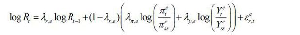
Various factors affect the monetary policy stance of the U.S. Directly incorporating the Federal Funds rate would bias our estimation, as the expected interest rate change can affect capital flows even before the actual changes. Therefore, it is necessary to control the information held by market participants at the time of the monetary policy. When the interest rate changes in the market, economic actors will act proactively, and this tendency becomes more pronounced in capital flows. For example, at the time the United States ended the zero-interest era and normalized her monetary policy, the actual rate hike took place in 2016, but because such normalization had been widely predicted before this event, U.S. Treasury bond yields began to rise starting at the end of 2015. Thus, subsequent capital reversals took place around the end of 2015. The actual increase in the interest rate due to the increase or decrease in the interest rate will be correlated with capital outflows before the actual increases in December of 2016. Several existing methods can be used to identify U.S. interest rate shocks, but this paper uses the relatively simple form of identification used by Iacoviello and Navarro (2019).7 It is straightforward, but we believe that it is very intuitive at the same time and that it is rigorous enough to identify monetary policy shocks. The following regression equation is utilized to identify the impact of interest rate hikes in the United States.

Here, rt is the U.S. Federal Funds rate, Zt denotes the control variables including current inflation rate and the log of the real GDP and corporate spreads in the U.S. We also include lagged values of the U.S. Federal Funds rate, the time trend and squared terms of the time trend. We use lagged variables of the last four quarters. Our series stretches from the third quarter of 1987, when Alan Greenspan was appointed as chairman of the Federal Reserve Board, to the most recent first quarter of 2019. It should be noted that in our main regression, our sample starts in 1995 due to data availability pertaining to the international investment positions of Korea. The shadow rate of Wu and Xia (2016) replaces the Federal Funds rate in the era of zero interest rates.
Figure 1 shows the U.S. monetary policy shocks identified through the regression equation. We find that the Federal Funds rate and the identified shocks can vary substantially depending on the period. In particular, starting in 2002, there is a stark difference between the two series.8 Ultimately, the series replicate and update the U.S. monetary policy shock of Iacoviello and Navarro (2019) up to the first quarter of 2019.
FIGURE 1.
IDENTIFIED U.S. MONETARY POLICY SHOCKS
Note: The solid line represents identified U.S. monetary policy shocks, and dashed line indicates changes in the Federal Funds rate. We identify U.S. monetary policy shocks by projecting the Federal Funds rate onto the information set of current and lagged macroeconomic variables, as in Iacoviello and Navarro (2019).
B. Data and the Econometric Methodology
The local projection method, initially proposed by Jordà (2005), has been used in various impulse-response analyses. The method does not require the specification of the structural relationships between variables in a dynamic system. Thus, it is known to have more flexibility and greater versatility than other methods that estimate systems of autoregressive variables, i.e., VARs. Accordingly, it has been very popular in recent years and has been applied especially when incorporating state dependencies. While it is popular due to its versatility, it also has shortcomings in that the number of samples decreases rapidly as the spanning of the impulse response increases. Thus, it can drop observations in a relatively short spanned sample.
Here, we consider the following regression equation,

where yt is the log stock of assets or liabilities, MSt is the identified U.S. monetary policy shock as described in the previous section, and Wt denotes the added control variables. The capital stock yt distinguishes foreign liabilities from residents’ assets and is further categorized into direct investments (FDI), portfolio investments, and other investments, as in financial accounts in the balance of payment process.
We note that the specification and selection of controls proceed similarly to Banerjee, Devereux, and Lombardo (2016). Control variables include current and lagged (up to two quarters) values of the real GDP growth rate, nominal exchange rate appreciation, real GDP growth rates of major trading partners, interest rate changes of one-year monetary stabilizing bonds, and percentage increase of foreign exchange reserves. The real GDP growth would capture the capital flows generated by additional production. Additionally, the domestic interest rate and nominal exchange rate fluctuation would capture exogenous variations in the yield may affect capital flows. The time trend and the dummy for the crisis periods are included as further controls.9 We presume that capital inflows by one type do not have any structural correlation with another. In other words, the regression equation of a certain type of capital flow does not have other types of capital flows as control variables.
In the above regression equation, βh is the elasticity of the h-period-ahead capital adjustment to a U.S. monetary policy shock. In a standard VAR, historical evolution and the consequent inference can be made by estimating a system of autoregressive variables. However, when doing so, the estimated coefficients of the model are not easily understood nor useful if one is interested in impulse and response factors. Instead, in local projections, the effect of the independent variable on the dependent variable is estimated by locally projecting the former onto the latter. It does not require specification of the true multivariate dynamic system. Thus, βh in our regression equation would convey a more intuitive interpretation of the system in terms of the impulse response coefficients. Indeed, Plagborg-Møller and Wolf (2020) argue that VARs and local projections will ultimately provide the same estimate if the data-generating functions are identical. That is, VAR (∞) and local projection would give an identical coefficient and confidence interval asymptotically.
In Figure 2, we plot the evolution of logged external assets and liabilities. Again, the international investment position data is only available after 1995, and our data extends from 1995q1 to 2019q3. We also note that mid-90s is the period of the beginning of financial liberalization. Starting in 1989, restrictions on external capital accounts slowly began to be released. Thus, it will be more appropriate to cut the periods before 1995 and focus only on the periods afterwards.
The upper left part of Figure 2 shows that external assets and liabilities increased quite dramatically before the global financial crisis. However, the pace of the growth slowed somewhat after the crisis for the foreign liabilities. Instead, external assets held by residents grow more rapidly. External assets swelled more compared to external liabilities by 2014q3, and Korea became a net external creditor after that point. From the figure, we can observe the importance of gross capital flows. It is increasingly important to understand the determinants of both the behaviors of residents and of international investors.
FIGURE 2.
EXTERNAL ASSETS AND LIABILITIES OF KOREA
Note: The solid line indicates the log of external asset holdings by residents. The dashed line represents the log of the foreign liabilities of foreign investors.
We can also confirm that both the FDI and other assets catch up with the external liability amount. FDI assets surpass this amount even before the global financial crisis. While the magnitude of portfolio assets is slightly smaller than that of the liabilities, the discrepancy between two is also narrowed dramatically. Again, in the regression equation, the dependent variable yt+h - yt-1 captures the difference between the h-period-ahead values of the log assets or liabilities and the values at t-1 . Additionally, the local projection method estimates the average dynamic responsiveness of the monetary policy on those distanced variables. The estimated coefficients can be interpreted as the monetary policy responses of external assets or liabilities.
Thus far, we have examined the stock of external assets and liabilities. In Figure 3, we instead plot the first differenced values of the log external assets and liabilities. Thus, these percentage changes of the stock of assets or liabilities map into capital flows of different types of assets or liabilities. We note the following: first, the capital flows of residents and international investors are highly correlated. The similarities between the two series are more pronounced in the portfolio flows than in the FDI.
FIGURE 3.
CAPITAL FLOWS (CHANGES OF EXTERNAL ASSETS AND LIABILITIES) OF KOREA
Note: The solid line indicates the log differences of external asset holdings by residents. The dashed line denotes the log differences of the foreign liabilities of foreign investors.
Second, the volatility of portfolio flows is greatest, while the volatility levels of FDI and other flows are less significant. Third, the overall volatility of capital flows is slightly subdued after the global financial crisis, but not by much. From the first two arguments, we can expect the impulse response of flows by residents and international investors to be alike, as in other studies of small open economies. In next section, we show that the impulse responses of total gross capital flows are mostly driven by portfolio flows. It is also important to note that the overall volatility does not decrease notably after the global financial crisis. Thus, any significant change in the elasticity of a U.S. monetary policy shock will be surprising.
IV. Empirical Results
A. Main Results
In this chapter we present our main empirical results. We split our sample periods into two sub-samples and run an impulse response analysis independently for each bin. We split our samples for the following reasons. With a U.S. monetary policy shock, we want to observe the gross withdrawals of capital flows in Korea, which are observed in many other countries. That is, we examine whether there are inflows by residents and outflows by foreigners along with a U.S. monetary policy shock. We report the results after running a regression on the entire sample in Appendix A. However, we could not recover the withdrawals of capital reported in other studies for the entire sample.
At the same time, we examine a possible structural break in the data-generating processes in different time periods. The inclusion of the great financial crisis periods could also deteriorate the overall results due to extreme capital flows or monetary policy shocks during these periods.10 Thus, in our baseline regression, we split our sample and presume that each sample period follows different data-generating processes and impulse responses.
Figure 4 shows the impulse responses to U.S. monetary policy shocks for domestic residents’ capital flows before the global financial crisis. As in Albrizio et al. (2019), we report 68 percent and 90 percent confidence bands; the dark band denotes the 68 percent band and the light band is the 90 percent error band.
FIGURE 4.
IMPULSE RESPONSES TO U.S. MONETARY SHOCKS FOR ASSETS BEFORE THE GLOBAL FINANCIAL CRISIS
Note: The figure shows the impulse responses to U.S. monetary policy shocks for the logged assets of residents. The sample ranges from 1995q1 to 2008q4. Light grey denotes the 90 percent confidence interval, while dark grey is the 68 percent confidence interval.
At the moment of a 100-basis-point U.S. monetary policy shock, the total amount of external assets by residents dropped by around 1.7 percent (of its previous stock). On average, there are small capital withdrawals by residents. The inflows last for two quarters, reaching 4.8 percent, and slowly return to the initial level afterwards. The magnitudes of capital inflows by residents are not statistically significant at the 90% confidence interval at the peak. Again, we will compare our results with foreign investors' impulse responses to determine whether the magnitude is larger in the responses of the stops, as in other countries.
The results vary if we focus more closely on the different types of capital flow by residents. Portfolio flows are most responsive to U.S. monetary policy shocks. When hit by a 100-basis-point shock, there are withdrawals by residents. Portfolio investments drop by 12.7 percent at that moment and further by 22.1 percent during the subsequent first quarter. Portfolio inflows are reversed in the second quarter and slowly rebound. For other flows, including banking flows, there are also capital inflows by residents. The magnitude amounts to 5.4 percent the third quarter after the shock. FDI flows also witness inflows of residents, but in a greatly delayed pattern. In summary, capital flows by residents are most notable in portfolio flows. While the magnitude and statistical significance are not very strong in the flows overall, those of the portfolio flows stand out noticeably.
Next we move on to the impulse responses of foreign investors. Figure 5 shows the results of the impulse responses to a U.S. monetary policy shock on capital flows by foreign investors before the global financial crisis. When hit by a 100-basis-point increase in U.S. monetary policy, foreign investors pull out their capital by around 6.0 percent (relative to its previous level). The capital outflows or withdrawals by foreign investors continue for up to two more quarters, and the magnitude amounts to 13.8 percent. The overall impulse is greater compared to the average withdrawal amount by domestic residents. Thus, we will observe net capital outflows on average when hit by an external U.S. monetary policy shock. The results are consistent with the standard narratives pertaining to average emerging economies.
Again, when further distinguishing between the types of flows, we find that the response is strongest for portfolio flows. The bottom left part of Figure 5 shows that with a one-hundred-basis-point increase in the U.S. monetary policy, portfolio outflows by foreign investors would reach 13.4 percent. The outflows amount to 28.9 percent after two quarters, after which they reverse. The response by the FDI flows also marks its lowest point during the second quarter, while the magnitude is not as strong compared to the portfolio flows. However, the responses of other flows, which include banking flows, are not very notable.11
FIGURE 5.
IMPULSE RESPONSES TO U.S. MONETARY SHOCKS ON LIABILITIES BEFORE THE GLOBAL FINANCIAL CRISIS
Note: The figure shows the impulse responses to U.S. monetary policy shocks for logged liabilities, i.e., the claims of foreign investors. The sample ranges from 1995q1 to 2008q4. Light grey indicates the 90 percent confidence interval, while dark grey shows the 68 percent confidence interval.
Next, we move on to the after-the-crisis subsample periods. As explained previously, many people argue that capital flows in Korea became more resilient. In Figure 6, we report the impulse responses to a U.S. monetary policy shock for residents’ assets. Again, there are contractions in total assets, and the pattern is driven by portfolio flows. In upper left part of the figure, we can observe that with a one-hundred-basis-point increase in the U.S. monetary policy, total assets would drop by 1.9 percent. The magnitude reaches 2.9 percent during the subsequent third quarter.
FIGURE 6.
IMPULSE RESPONSES TO U.S. MONETARY SHOCKS FOR ASSETS AFTER THE GLOBAL FINANCIAL CRISIS
Note: The figure shows the impulse responses to U.S. monetary policy shocks for the logged assets of residents. The sample ranges from 2010q1 to 2019q2. Light grey shows the 90 percent confidence interval, while dark grey shows the 68 percent confidence interval.
While the inflows are similar at the moment of the shock, subsequent flows are much smaller than they were before. In portfolio flows, the inflows amount to 9.9 percent during the third quarter after the shock. We note that the scale on the y axis is much large for portfolio flows than for any of the other flows. We claim that the overall pattern is again driven by portfolio flows, but at a much lower magnitude than in the before-the-crisis period.
Moving forward to the foreign investor’s side in Figure 7, we also do not see any significant contractions in the total claims with those beforehand. At the moment of a 100-basis-point U.S. monetary policy shock, overall claims by foreign investors decrease by 4.4 percent. They drop further by as much as 4.8 percent and then rebound afterward. However, this outcome is not statistically significant at the 90 percent confidence level. In agreement with all other analyses, portfolio flows are the main drivers of the overall flows by foreign investors. However, the magnitude of withdrawal at the moment of the U.S. monetary policy shock is 5.6 percent, and then 5.7 percent in the following quarter. Compared to 13.4 percent and 19.9 percent, the magnitudes are much smaller. For FDI and other flows by foreign investors, there are not statistically significant responses at the moment of a U.S. monetary policy shock. Other flows show slight increases after six quarters, but again the results are not statistically significant at the 90 percent confidence level.
FIGURE 7.
IMPULSE RESPONSES TO U.S. MONETARY SHOCKS ON LIABILITIES AFTER THE GLOBAL FINANCIAL CRISIS
Note: The figure shows the impulse responses to U.S. monetary policy shocks for logged liabilities, i.e., the claims of foreign investors. The sample ranges from 2010q1 to 2019q2. Light grey indicates the 90 percent confidence interval, while dark grey shows the 68 percent confidence interval.
At this stage, let us compare the impulse responses of the two different sample periods together. In Figures 8 and 9, we combine all of the figures presented earlier. We note that the dashed line here indicates the results for the before-the-crisis sample, while the solid blue line represents the after-the-crisis sample. In Figure 8, we find that retrenchments in assets are notable, especially with regard to portfolio assets before the crisis. However, the results are not preserved in the after-the-crisis period. Again, it is difficult to claim that patterns by domestic investors show any withdrawal of assets overall upon a U.S. monetary policy shock. For portfolio assets, a main component of capital flows reacting to U.S. monetary policy, we can observe some degree of inflow by residents. Nonetheless, the magnitude compared to the before-the-Crisis period are again less than half. We find that the overall responsiveness is dwarfed after the crisis.
FIGURE 8.
IMPULSE RESPONSES TO U.S. MONETARY SHOCKS FOR ASSETS BEFORE AND AFTER THE GLOBAL FINANCIAL CRISIS
Note: The figure shows the impulse responses to U.S. monetary policy shocks for the logged assets of residents. The solid blue line indicates the results from the after-the-crisis period (2010q1--2019q2), and dashed line denotes the results from the before-the-crisis period (1995q1—2008q4). Here, the 90 percent confidence intervals are reported.
Figure 9 shows that the magnitude of withdrawals by foreign investors is also less than half that in after-the-crisis sample. While the level of foreign claims does not recover to the initial level after six quarters in the before-the-crisis sample, the blue line returns to the initial level relatively quickly. These results are mostly driven by portfolio flows. We note that the scales of the figure for portfolio flows are twice as large as that of the overall figure. While there is more than a 28 percent decrease in portfolio flows in the before-the-crisis, sample, those in the after-the-crisis sample do not exceed six percent throughout. We also note that the 90 percent error band of the impulse response in the after-the-crisis sample does not overlap with the impulse response of the before-the-crisis sample.
FIGURE 9.
IMPULSE RESPONSES TO U.S. MONETARY SHOCKS ON LIABILITIES BEFORE AND AFTER THE GLOBAL FINANCIAL CRISIS
Note: The figure shows the impulse responses to U.S. monetary policy shocks for the logged assets of residents. The solid blue line indicates the results from the after-the-crisis period (2010q1--2019q2), and dashed line denotes the results from the before-the-crisis period (1995q1—2008q4). Here, the 90 percent confidence intervals are reported.
We note that the figures overlay the results of the two different samples. Thus, one cannot draw any statistical inferences based on our results. Our results are on average consistent with the prior hypothesis that the responsiveness of capital flows due to a shock is weaker in the after-the-crisis period. As we do assume that each periods follows a different data-generating process with different coefficients for all other controls, statistical inferences or tests could not be realized from the figures. We also add a couple of robustness checks in the appendix, including a specification incorporating the VIX or a different time trend. These results are broadly consistent with our baseline results.
Lastly, we compare the results between the current article and the results in Choi (2020). In a companion paper, Choi (2020) documents the effects of the U.S. monetary policy on gross capital flows, an analysis similar to ours. While asking the same question, current article uses the log stock of assets and liabilities, but Choi (2020) uses capital flows normalized by quarterly GDP. Also, current one focuses on the dynamic (h-periods apart) log changes of assets and liabilities. However, the specification in the companion article uses the spontaneous flows (capital flows normalized by the quarterly GDP) as the dependent variables. The different types of normalization and the different specifications yield somewhat different results. First, though Choi (2020) also finds marginally decreased elasticity of capital flows after the crisis, the results are mainly driven by other flows, which include banking flows. Indeed, with the different normalization process, overall volatilities are greater in the other flows and the marginal elasticity of the flows to a U.S. monetary policy shock is larger than in the portfolio flows. It is not possible to claim that one specification outperforms the other. A different normalization method implies a different anchor by which to measure the percent or the percentage change of capital stock. The current article uses the percent change compared to its own level of stock, while the previous article uses the percentage change over the GDP level as the basis for the analysis.
Thus, our baseline results and consequent claims possibly depend on the specification used. Indeed, the lack of robustness in the impulse response analysis of a monetary policy shock is well known and widely debated.12 Although we confirm our main message in our baseline regression results, we admit that our results may vary if we apply another specification, e.g., the number of lags included, other controls, etc. Choi (2020) also document an extensive robustness analysis, concluding that the results may vary if a different specification is used or if including other control variables.
V. Financial Friction and the Elasticity of Capital Flows
Thus far, we have empirically analyzed the impact of U.S. monetary policy shocks on capital flows in Korea. In particular, we confirmed that in our baseline regression, the marginal responses of capital flows have been far less notable in the sample periods after the global financial crisis. In this section, we seek possible explanations for the previous empirical results.
We conjecture that if financial friction, which has been claimed as the main source of external vulnerability and the consequent volatile capital flows, can be improved, the responsiveness could decrease. Korea has passed through various macroeconomic transitions after the global financial crisis. As shown in Figure 2 and Figure 3, the accumulation of assets has outpaced liabilities. Since 2014q3, external assets held by residents do exceed claims by international investors. Among others, we focus on institutional changes in financial friction. We examine the theoretical model and determine whether these improvements of financial friction may be replicated in the empirical results in the previous section; if the fraction of net worth that can be pledged is increased when the Korean financial sector borrows from outside, it should follow that the elasticity of the outflow decreases.
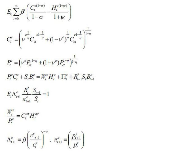
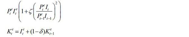
A. A Two-Country New Keynesian Model with Financial Friction
Banerjee, Devereux, and Lombardo (2016) construct a two-country new Keynesian model (center (core) and the periphery) with financial friction. They focus on the derivation of optimal monetary policies with international cooperative stances. However, a basic model was applied in other studies, such as Devereux, Engel and Lombardo (2020), who derive implementable monetary policy rules, for instance. Here, we do not focus on any changes in monetary policy, nor on whether it became cooperative or not after the global financial crisis. Instead, we utilize the simplest form of monetary policy, Taylor rules, in their model, and vary the degree of financial friction that governs leverage constraints.
Because we use the same model used as in Banerjee, Devereux, and Lombardo (2016) and Devereux, Engel, and Lombard (2020), we abstract from the details of the model.13 We also note that as in the original paper, we abstract from quantitative exercises. The model's intuition is as follows. In the model, there are two countries; the core and the periphery. Central banks in each country operate their respective monetary policies according to the Taylor rule, and there is Calvo-type price rigidity. The core households will issue a one-period risk-free bond, and the households of the periphery will attempt intertemporal consumption-smoothing through bonds issued by the core households. Companies in each country combine labor and capital to produce core and peripheral products, respectively. Households in each country will consume final goods that combine consumer goods from their own and other countries. These are the assumptions of a standard two-country model.
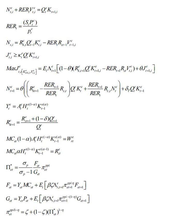
In addition, we also assume the following types of financial friction. Instead of a household owning capital and lending it directly to firms, a bank exists as an intermediate.14 Banks have equity capital and can additionally borrow, but only a certain fraction of their net worth. Thus, there is a leverage constraint. The core bank borrows from the core household considering their net worth, purchase capital goods and loan those to the firms in the core country. In addition, the core bank also loans a fraction of its funds to banks of the peripheral countries. Periphery banks borrow capital from the core banks, along with their own capital. They then purchase capital goods and rent those to firms in the periphery. For convenience, we assume that a bank in the periphery does not receive any funds from its own households. In this structure, the households of the periphery hold bonds from the core households. The core households receive funds by issuing assets to periphery households and then rent those to the core banks, who will finance the banks in the periphery and firms in the periphery eventually. With this system, we can determine the gross capital flows between the two countries.
The model with financial friction in the banking sector has the following discrepancies compared to the standard model. If there is a monetary policy shock in the core economy, the leverage constraints in the bank will be tightened and the spread between the interest rate for funds borrowed by the company and the interest rate of the risk-free bond will increase. As a result, capital is not sufficiently brokered and is not sufficiently transferred to production. In addition, as the amount of funded capital decreases, core investors reduce their amounts of capital invested in peripheral countries. In other words, foreign claims will decrease with monetary policy shock. The impact of this increase in core interest rates leads to a decrease in the income of the peripheral households due to the general equilibrium effect. The peripheral households sell foreign assets, and the periphery residents’ capital invested abroad then decreases.
Regarding the impact of a US rate hike, the model creates inefficiency in financial
intermediation, and such factors are greatly amplified by the impact of capital inflows.
From a resident’s point of view, leverage constraints and an increase in spreads are
the most important causes of volatility in capital outflows. In the model, the parameters
of these leverage constraints are denoted by Kt. In the original paper, the stochastic processes Kt of the two countries are identical. On the other hand, in this paper, we assume that
each country has processes with different mean value parameters. Thus, our presumptions
during these thought experiments are as follows: during the period before the global
financial crisis, Korea, i.e., the periphery, has a smaller value than a developed
country. However, after the global financial crisis, there is an improvement in the
credibility of Korean borrowers, and fractions of net worth that can be pledged are
enhanced.  increases and the degree to which leverage is restricted is lowered.
At this point, we examine the responses of periphery household’s assets and core household’s assets (liabilities of the periphery) upon a core rate hike. The leverage constraints of core banks have a value of 0.45 both before and after the global financial crisis. Core banks can borrow 45% of their equity value from households. However, the leverage constraint of peripheral banks has a value of 0.38 before the global financial crisis and is then enhanced to 0.45 thereafter. Periphery banks can borrow 38% of the value of capital from core banks beforehand. These restrictions will be increased to 45% after the global financial crisis due to the institutional improvement. If the inefficiency of financial intermediation is reduced, the impact of the interest rate hike on the core will also be lower.
With an enhanced value of Kt, the core monetary policy hike will not be transmitted to periphery economies as much as before. As a result, loans from core banks to peripherals decrease by less. The income decrease by periphery households due to the interruption in financial intermediation would also be less severe. The assets that the peripheral households withdraw from the core households will be smaller as a result.
The results of these simulations are reported in Figure 10. The Y axis represents the deviations from the steady-state values. We find that
the impact of a rate hike in the core country (U.S.) reduces foreign assets in both
countries. However, there are discrepancies between different values of s. The solid blue line shows the impulse responses with an increase in , while the dashed line shows the impulse responses with the previous value of . Again, a larger indicates an improvement in institutional friction and thus applies to after-the-crisis
periods. We also find that for the blue solid line, there is less deviation from the
steady state due to the impact as compared to that indicated by the black dashed line.
That is, there is less responsiveness in the reallocation of assets than beforehand.
With the improvement in foreign investor’s credibility and the improved pledgeability
for the given value of net worth, spillover from the U.S. monetary policy becomes
weaker.
FIGURE 10.
IMPULSE RESPONSES TO A MONETARY POLICY SHOCK IN A CENTER COUNTRY PERIPHERY
Note: The figure shows the external positions of the periphery and the center economies relative to each other. Total assets of the center will be a liability to Korea. The blue line denotes the impulse response of a center monetary policy shock with increased leverage constraints.
B. Other Possible Answers, International Trilemma and Independence of Monetary Policy
To this point, we find that institutional changes in financial intermediations may explain the lower level of responsiveness of capital flows to a U.S. monetary policy shock. However, there could also be many other culprits.
Along with various macroeconomic transitions, it is possible that in different circumstances, policies which govern the responsiveness of capital flows to U.S. monetary policy shocks have changed. Currently, there are many studies documenting optimal monetary policy responses to foreign capital inflows. An optimal monetary policy which simultaneously determines the optimal exchange rate policy depends on domestic fundamentals, such as dominant currency pricing and financial friction.15 With the altered external circumstances, monetary policy may have changed as well. At the same time, macro-prudential policies or capital controls have been adopted since the global financial crisis, and those may have been effective since that time.
Indeed, Korea may not be the only country that has undergone a transition with regard to international capital flows. Shin (2014) claims that while the first phase of global liquidity was marked by banking flows, the second phase of global liquidity after the global financial crisis is now marked by bond flows, especially debt securities. Possibly, it is more of what is termed push-side transitions than their pushside counterparts. Avdjiev et al. (2020) noted that the overall marginal response of capital flows based on U.S. monetary policy rose substantially due to the 2013 Fed’s ‘taper tantrum’, and then reverted. They claim that the change in the responsiveness was mainly driven by increases in the lending shares of more capitalized banking systems. Forbes and Warnock (2020) claim that extreme capital flow movements themselves have not increased since the global financial crisis. At the same time, extreme capital flow movements are less correlated with changes in global risks.
Even if we are not sure of the true cause of the change in vulnerability of capital flows, we can discuss possible influences on monetary policy, especially the independence of monetary policy. One of the most cited propositions in international economics is the international impossible trinity. The trilemma argues that the opening of the capital market, the independence of monetary policy, and a fixed exchange rate cannot be achieved simultaneously. A small open economy which operates a fixed exchange rate system and has a high degree of openness in the capital market has significant limitations in terms of monetary policy operations.
Market participants are empirically testifying that Korea's capital outflows are strong against external shocks. Reflecting this situation, the IMF's Article IV report evaluated Korea's financial assets as safe assets according to such a situation. If this change in the trend is true, it will be possible to secure considerable independence of monetary policy operations. It is possible to focus more on internal problems during the operation of monetary policy. Further discussions and research are needed to determine whether this resilience actually exists.
VI. Conclusion
In this article, we document the effects of U.S. monetary policy shocks on gross capital flows in Korea. External shocks are typically the main sources of vulnerability in an open economy. Especially in Korea, several waves of capital inflows and subsequent sudden withdrawals have caused severe fluctuations. To understand the effects of U.S. monetary policy shocks, which are claimed to have caused the global financial crisis, not only foreign capital flows but also residents’ capital flows should be the lynchpin of monetary and fiscal policies.
We show that first in Korea, as in other small open economies, not only net but also gross capital flows matter. When U.S. monetary policy shocks increase, foreign and domestic investors withdraw their positions in Korea and in other parts of the world, respectively. Consistent with people’s prior behavior, the elasticity of capital flows have changed since the global financial crisis. We explore the possibility of an institutional improvement on financial friction. If the amount to pledge against foreign investors has increased, the responses of both types of investors would decrease upon a monetary policy shock of the core economy, i.e., the U.S.
We claim that our findings could serve as guidance for monetary or exchange rate policymakers. However, we also claim that our reasoning is only suggestive at this moment. Further evidence is needed. Especially for institutional change, micro-level data (loan level and covenant) are needed, though this remains as a future research agenda.
Appendices
APPENDIX
A. Robustness Checks
1. Empirical Results: All Periods
In this section, we present the impulse responses of U.S. monetary policies in the form of gross capital flows for all sample periods. In our baseline specification, we split our sample into two bins, before and after the crisis, and analyze each bin independently. The results therein are similar to those analyzed for panel data, for example in Banerjee, Devereux, and Lombardo (2016).
One may instead be interested in running the entire sample while including the global financial crisis period. Consequently, in the appendix, we report the results for this specification. We include a crisis dummy for both the global financial crisis and the East Asian Crisis; the crisis dummy is one for 2008q1-2009q2 and 1997q4-1998q1. Our results are reported in Figure A1 and Figure A2. Unlike the baseline results in section 4, we do not see capital inflows by residents (decrease in assets), nor capital outflows of foreign investors (decrease of liabilities). In Figure A1, capital flows by residents show consistent increases with U.S. monetary policy shocks. This pattern does not vary with different types of flows. Also in Figure A2, we see consistent increases of foreign flows with U.S. monetary policy shocks. The results do not vary even if we include squared time trends as a further control. Overall, we could not recover the patterns observed in other studies.
We conjecture that there is a break in the time trend before and after the crisis. Thus, it is possible that outflows by foreign investors and inflows by residents, which are widely reported in other emerging economies, are only observed if we split the sample and apply different time trend for both economies.
2. Empirical Results: with VIX
In this chapter, we report the results of a specification with the VIX and drop the appreciation of nominal exchange rates. We exclude the VIX as a control in our baseline analysis, as the global risk aversion captured by the VIX can fluctuate due to U.S. monetary policies. Thus, to include the VIX as an extra control while incorporating the shock itself may lead to endogeneity issues. At the same time, it is also possible that there are orthogonal deviations of the VIX with U.S. monetary policies. Thus, we utilize a specification which includes the VIX as a control. Also, we exclude nominal exchange rate appreciation as a control. As a small open economy, the baseline specification presumes that exchange rates vary along with external sources and thus form an exogenous variable. However, it is also plausible that nominal exchange rates are determined endogenously. In a new specification, we exclude nominal exchange rate appreciation and include the VIX as a control. Figure A3 and Figure A4 shows the results.
Overall, our main message is not altered. For capital flows by domestic residents, the declines in the total flows are lower in the after-the-crisis bins. However, the discrepancies are not very notable. On the other hand, portfolio flows show clearer distinctions between the two. While there is a clear hump shape in the before-the-crisis sample, no clear pattern is observed in the after-the-crisis sample. For the foreign capital flows shown in Figure A4, the results are less stark between the samples before and after the crisis. However, the overall images are very similar; the average responses of foreign outflows are weaker than before, and the results are mainly driven by portfolio flows.
FIGURE A3.
IMPULSE RESPONSES TO U.S. MONETARY SHOCKS FOR ASSETS BEFORE AND AFTER THE CRISIS, WITH THE VIX
FIGURE A4.
IMPULSE RESPONSES TO U.S. MONETARY SHOCKS FOR LIABILITIES BEFORE AND AFTER THE CRISIS, WITH THE VIX
3. Empirical Results: Other Time Trends
One can expect that the upward or downward pattern can be controlled by with the added t-squared trend. That is, if further controlling a hump-shaped pattern, one may find different implications of the impulse response patterns.
Here, we report the outcomes with the t-squared term included. Again, our overall message does not change. Foreign capital outflows are mostly notable with a U.S. monetary policy shock, and this response is mostly driven by portfolio flows. While there is less of an upward or downward trend in the FDI or other flows, the results do not alter our overall picture.
4. Empirical Results: Interacting with the Crisis Dummy
It is also possible for capital flows to have different responses to a monetary policy shock. Thus, in this chapter we incorporate a crisis dummy with a monetary policy shock for the sample period before the global financial crisis. Here, we utilize two periods: the East Asian Crisis (1997q4-1998q1) and the financial turmoil due to the IT bubble (2003q1-2003q2). Additionally, the new specification only changes the results for before-the-crisis sample, and the results will be identical for the after-the-crisis sample period. Figures A7-A8 correspond to Figures 4 and 5 in our main body. Unfortunately, the results do not vary much from our baseline regression. There is no significant chance in the impulse responses of the monetary policy (during the non-crisis state), and the confidence intervals are still very wide and robust. Thus, to mute the large swings during the crisis state, it appears to be sufficient to put a wedge in the capital flows during periods of turmoil.
FIGURE A5.
IMPULSE RESPONSES TO U.S. MONETARY SHOCKS FOR ASSETS BEFORE AND AFTER THE CRISIS, WITH THE T-SQUARED TREND
FIGURE A6.
IMPULSE RESPONSES TO U.S. MONETARY SHOCKS FOR LIABILITIES BEFORE AND AFTER THE CRISIS, WITH THE T-SQUARED TREND
B. Full Set of Equations for the Model Simulations
We supplement the full set of equations to simulate Banerjee, Devereux, and Lombardo (2016). It should be noted that we simply assume the Taylor rule as a monetary policy both for core and center economies. Thus, the current set of equations consists of equations from the simplest model presented in Banerjee, Devereux, and Lombardo (2016). Please see Banerjee, Devereux, and Lombardo (2015) for a more in-depth description of the system of equations.
1. Households’ Problem
2. Capital Goods Producers’ Problem
3. Emerging Market Economies Banks’ Problem
4. Monetary Policy
5. Center Country’s Optimization Problem
6. Center Country Banks’ Problem

Notes
This paper is based on Choi, Woo Jin, 2020(forthcoming), “Effect of US Monetary Policy on Gross Capital Flows: Cases in Korea,” KDI (in Korean). Results change as data and the specification changes. Soyeon Ahn provided outstanding research-assistance.
Furthermore, Miranda-Agrippino and Rey (2020) also claim that it is not feasible to cope with those by means of conventional monetary policy or exchange rate policies.
For further discussions on gross capital flows and the related terminology (surges, flights, stops, and retrenchments) please see Forbes and Warnock (2012).
We note that these results are even different from the results of the companion article, Choi (2020). In the previous article, preceding the current article, most of the stand-out results are for other (banking) flows. We will discuss this difference later in sections IV and V.
It should be noted that we do not provide statistical test results that confirm the differences. One cannot directly map and compare the confidence intervals of the two different samples. Thus, we posit no statistical inferences.
In Iacoviello and Navarro (2019), the authors examine the impact of U.S. interest rate shocks on GDP in developed and emerging economies. Utilizing a panel local projection approach with a vulnerability index, they conclude that U.S. interest rate shocks are negatively transmitted to neighboring countries but that the degree of spillover depends on a certain vulnerability index, such as the exchange rate system, degree of trade openness, or other instability indicators.
We note that Devereux, Engel and Lombardo (2020) also use a version of the model in Banerjee, Devereux, and Lombardo (2016) to derive an implementable monetary policy.
Iacoviello and Navarro (2019) provide a simple but intuitive methodology with which to identify monetary policy shocks. We also have attempted high-frequency identification using Federal Funds futures. However, the necessary data is only available for very recent periods.
A shock in the form of a significant spike in the US interest rate is observed in the first quarter of 2009, while this is not seen in changes in simple interest rates. We note that in our baseline regression, we exclude the sample period of 2009, which contains extreme U.S. interest rate shock increases. This does not alter our main results.
The crisis dummy is one for 2008q1-2009q2 and 1997q4-1998q1. Here, we split the sample before and after the crisis, dropping the period of 2009 from our entire analysis in our baseline specification.
We note that in the companion paper of Choi (2020), the baseline regression includes the entire sample.
On average, banking flows are said to have the most responsive results when hit by an external shock. Albrizio et al. (2019), which covers banking flows, reports around a 12 percent decrease in the second quarter. Also, Choi (2020) reports the most responsive results in banking flows. Unlike those studies, in our baseline specification, we did not observe any significant results in other flows.
References
, , & . (2016). Self-Oriented Monetary Policy, Global Financial Markets, and Excess Volatility of International Capital Flows. Journal of International Money and Finance, 68, 275-297, https://doi.org/10.1016/j.jimonfin.2016.02.007.
, , , & (2013). Gross Capital Flows: Dynamics and Crises. Journal of Monetary Economics, 60(1), 113-133, https://doi.org/10.1016/j.jmoneco.2012.12.004.
, & . (2015). Capital Flows and the Risk-Taking Channel of Monetary Policy. Journal of Monetary Economics, 71, 119-132, https://doi.org/10.1016/j.jmoneco.2014.11.011.
, , & . (2017). If the Fed Sneezes, who Catches a Cold? Journal of International Economics, 108, S23-S41, https://doi.org/10.1016/j.jinteco.2017.01.002.
, , & . (2020). Implementable rules for international monetary policy coordination. IMF Economic Review, 68(1), 108-162, https://doi.org/10.1057/s41308-019-00104-1.
, & (2012). Capital Flow Waves: Surges, Stops, Flight, and Retrenchment. Journal of International Economics, 88(2), 235-251, https://doi.org/10.1016/j.jinteco.2012.03.006.
. (2012). Capital Flows, Push versus Pull factors and the Global Financial Crisis. Journal of International Economics, 88(2), 341-356, https://doi.org/10.1016/j.jinteco.2012.05.003.
, & . (2019). Foreign Effects of Higher US Interest Rates. Journal of International Money and Finance, 95(1), 232-250, https://doi.org/10.1016/j.jimonfin.2018.06.012.
. (2005). Estimation and Inference of Impulse Responses by Local Projections. American Economic Review, 95(1), 161-182, https://doi.org/10.1257/0002828053828518.
, & (2004). A New Measure of Monetary Shocks: Derivation and Implications. American Economic Review, 94(4), 1055-1084, https://doi.org/10.1257/0002828042002651.
, & . (2016). Measuring the Macroeconomic Impact of Monetary Policy at the Zero Lower Bound. Journal of Money, Credit and Banking, 48(2-3), 253-291, https://doi.org/10.1111/jmcb.12300.
. (2018). Analysis of Changes in Determinants of Foreigners’ Bond Investment before and after the Global Financial Crisis: The Case of Korea. Journal of Money & Finance, 32(3), 101-128, in Korean, https://doi.org/10.21023/JMF.32.3.4.