
Assessing Alternative Renewable Energy Policies in Korea’s Electricity Market†
Abstract
This paper, focusing on the renewable portfolio standard (RPS), evaluates alternative renewable energy policies. We propose a tractable equilibrium model which provides a structural representation of Korea’s electricity market, including its energy settlement system and renewable energy certificate (REC) transactions. Arbitrage conditions are used to define the core value of REC prices to identify relevant competitive equilibrium conditions. The model considers R&D investments and learning effects that may affect the development of renewable energy technologies. The model is parameterized to represent the baseline scenario under the currently scheduled RPS reinforcement for a 20% share of renewable generation, and then simulated for alternative scenarios. The result shows that the reinforcement of the RPS leads to higher welfare compared to weakening it as well as repealing it, though there remains room to enhance welfare. It turns out that subsidies are welfare-inferior to the RPS due to financial burdens and that reducing nuclear power generation from the baseline yields lower welfare by worsening environmental externalities.
Keywords
Electricity Market, Renewable Portfolio Standard, Technology, Renewable Energy Certificate, Welfare
JEL Code
Q21, Q28, Q31
I. Introduction
In July of 2017, the new government of South Korea announced its policy goal, termed Renewable Energy 3020 (RE3020), which involved increasing the share of renewable power generation, which was 7% in 2016, to more than 20% by 2030.1 Later, in December of 2017, the Ministry of Trade, Industry and Energy (MOTIE) unveiled its Implementation Plan for RE3020. It proposes to expand public and private large-scale projects by enhancing local acceptability, where 95% of new power generation facilities will be based on solar and wind power. Subsequently, MOTIE issued the 8th Basic Plan for Long-Term Electricity Supply and Demand (MOTIE, 2017) which specifies the aggregate capacity and generation schedules for power sources from 2017 to 2031. Specifically, in the plan, the share of renewable energy generation, counting business-purpose generation only, becomes 20% by 2030, and it reaches 21.6% when adding self-consumption-purpose generation.
In terms of scale, RE3020 heavily relies on the expansion of business-purpose renewable power generation. As a main vehicle to achieve this goal, the government plans to strengthen the renewable portfolio standard (RPS). The promotion of renewable generation under RE3020 has fundamental significance in terms of i) ultimately improving environmental problems caused by greenhouse gases (GHG) and air pollutants, and ii) improving the nation’s energy independence through energy diversification. On the other hand, one can figure that if the obligation under the RPS is strengthened drastically to meet the RE3020 target, the burden of compliance may eventually be reflected in the retail electricity price and then passed on to consumers. At the same time, this concern can be relieved to a certain degree when considering that the latest forecast by the International Renewable Energy Agency (IRENA, 2018), grid parity—the price of renewable energy is equal to that of existing power sources—will not be long due to the cost reduction from technology development. After all, it is not an easy task to determine the overall welfare effects of the currently planned RPS reinforcement. This is also true when estimating the effects of renewable energy policies as alternatives to the current policy.
In this paper, we propose a competitive equilibrium model designed to evaluate alternative renewable energy policies, including RE3020. The model provides a structural representation of Korea’s electricity market, including its energy settlement system and renewable energy certificate (REC) transactions. Arbitrage conditions are used to define the core value of REC prices to identify relevant competitive equilibrium conditions. The model considers R&D investments and learning effects that may affect the development of renewable energy technologies. The model is parameterized to represent the baseline scenario under the currently scheduled RPS reinforcement and then simulated for alternative scenarios. As well as market effects, how the distributional effects of certain welfare factors—government net income, consumer surplus, producer surplus, and environmental effects—differ among alternatives is also examined.
It is found that achieving a 20% share of renewable energy generation via the RPS increases social welfare compared to the absence of the RPS. To be specific, from its absence, the introduction of the RPS results in an increase of the retail electricity price, thus hurting consumers. On the other hand, as nonrenewable energy generation shrinks, there is a significant decrease in externality costs. Overall, welfare is higher under the RPS. Furthermore, there is room for enhancing welfare through an additional strengthening of the RPS. It turns out that such welfare ranking remains the same throughout various sensitivity analyses. In addition, a simple production subsidy for renewable generation can achieve the target share of renewable generation under the RPS, but it is found to be inferior to the RPS in terms of overall welfare due to the high financial burden borne by the government. Next, if reducing nuclear power generation from the baseline, welfare is lowered due to the increased environmental externality costs caused by the expanded generation from fossil fuels, which overwhelms any reduction in nuclear accident costs.
The rest of the paper proceeds as follows. Section II provides a literature review as well as a historical background of relevant policies. In Section III the model is described, followed by Section IV, where the model is parameterized using various sources of data. Simulation results are shown in Section V, and Section VI concludes the paper.
II. Background and Literature
After two oil crises in the 1970s, the government enacted the Act on the Promotion of the Development of Alternative Energy in 1987 and established the Basic Plan for the Development of Alternative Energy Technologies (1988-2001) in order to diversify Korea's energy sources. Since the United Nations Framework Convention on Climate Change (UNFCCC) in 1992, various efforts to reduce GHG emissions have been made, and the commercialization of developed technologies has progressed gradually. In 1997, the Act on the Promotion of the Development Alternative Energy was revised as the Act on the Promotion of the Development and Use of Alternative Energy, by which the use and diffusion of alternative energy was actively promoted.
In 2002, the government set a target share of alternative energy generation within total electricity generation. In addition, under the Feed-in Tariff (FIT), renewable-based producers begun to receive price support when the market price dropped below the standard price through government contracts lasting 15 to 20 years. Thereby, renewable-based producers were able to sell electricity at a fixed price, greatly reducing market uncertainty and ultimately leading to the formation of an early renewable energy generation market. Despite the improved policy support, as the financial burden caused by the FIT grows, discussions focusing on the introduction of the RPS started. The introduction of the RPS was considered beneficial in comparison to the FIT in terms of: i) inducing technology development based on market principles, ii) responding to the UNFCCC, and iii) fostering industries by expanding the renewable energy market. In the end, the government enacted what was termed the Renewable Portfolio Agreement (RPA) as a pilot project for 2009-2011, implementing the RPS in 2012 with the abolition of the FIT.
The RPS obligates producers who are based on nonrenewable sources to supply an additional amount, in general calculated by multiplying nonrenewable generation by the supply-obligation rate, using renewable sources. In order to comply with this obligation, the obligated party can (partially) choose self-generation or external procurement. To illustrate this, for each 1MWh of renewable generation, a REC, which can be submitted to prove compliance, is granted, and by selling RECs producers can make up their additional costs. At the same time, one can purchase RECs and use them to prove their compliance. Either approach is legitimate under REC market transaction rules.
In July of 2017, the new government released the Five-Year Plan for National Administration, incorporating RE3020. RE3020 aims to raise the share of renewable generation, which was 7% in 2016, to 20% by 2030, mainly by applying higher supply-obligation rates for business-purpose generation. Table 1 shows the historical changes of the RPS supply-obligation-rate schedule. RE3020 plans to avoid biomass and waste-based development and to supply more than 95% of new generation facilities with solar and wind power in the future. Figure 1 shows MOTIE’s (2017) projected generation for 2017-2031 together with the actual generation for 2005-2016. In 2030, the share of business-purpose generation accounts for 20% (126 TWh), while it was 6.2% in 2017. Regarding domestic generation potential, Lee, Jo, and Yoon (2014), by considering technology development and physical area conditions, estimate these values to be 311 TWh for 2015 and 314 TWh for 2030. Such generation potential rates represent 54% of the total generation for 2017 and 47% of the projected total generation for 2030.
TABLE 1
RPS SUPPLY OBLIGATION RATE
Note: New provision in Sep 2010, first revision in Mar 2015, second revision in Dec 2016, Renewable Energy 3020 in Jul 2017.
Source: Enforcement Decree of the Act on the Promotion of Development, Use and Diffusion of New and Renewable Energy, Annex 3; National Planning Advisory Committee (2017).
FIGURE 1.
RENEWABLE ENERGY GENERATION: PAST AND FUTURE
Source: Korea Energy Agency, New and Renewable Energy Center, New and Renewable Energy Supply Statistics (https://www.knrec.or.kr/pds/st atistics.aspx, accessed Nov 19, 2018); MOTIE (2017).
Mandated policies, such as the RPS or the Renewable Fuel Standard (RFS), stipulate production in a way that is considered to have a high non-market value despite low profitability. As a result, introducing the RPS affects the generation mix as well as wholesale and retail prices by affecting supply-side incentives. In this sense, there has been a line of literature to analyze the economic impact of an RPS together with related energy and environmental policies. Kydes (2007) sought to analyze the impact of increasing renewable generation by 20% through an RPS in the United States. The National Energy Modeling System (NEMS) of the US Energy Information Administration (EIA) was used for the simulation. As a result, if implementing an RPS there, the elasticity cost is increased by 3% and the total electricity consumption is decreased by 0.6%. On the other hand, GHG emissions were 16.5% less than those in the absence of an RPS.
Fischer and Newell (2008) analyze the relative welfare effects of environmental policies—an RPS, renewable generation subsidies, carbon taxes, emissions trading, and R&D investment support. Specifically, their competitive equilibrium model consists of two stages, where R&D investment in the first stage induces a cost reduction in the second stage, and it is simulated to compare the performance outcomes of alternative policies. Considering GHG emissions as the cause of environmental externalities, they compare social welfare when each policy option achieves the same GHG emission reduction target. They found that the use of a carbon tax is least likely to decrease welfare, followed by emissions trading systems, an RPS, and R&D support. Fischer, Preonas, and Newell (2017) extend the model of Fischer and Newell (2008) to simulate policy alternatives after proposing a model that takes into account demand-side efficiency improvements. Compared to Fischer and Newell (2008), nuclear and hydropower are considered as additional endogenous sources, while renewable energy is subdivided into solar and others. Their analysis found that carbon taxes are most efficient among various policy options, achieving a 40% reduction of GHG emissions.
On the other hand, Bhattacharya, Giannakas, and Schoengold (2017) analyze the welfare effects of an RPS in a situation where consumers could purchase both general and renewable-energy electricity separately. Using a partial equilibrium model considering heterogeneous consumer preferences, simulations are carried out under the assumption of exogenous RPS-induced cost reductions. It was found that the introduction of an RPS increases consumer surplus for those who prefer eco-friendly electricity. Other results regarding prices, the total supply, and overall social welfare are found to depend on assumptions about consumer preferences and the degree of the price increase for renewable-energy-based electricity under an RPS.
Focusing on South Korea’s circumstances, Kim and Moon (2005) examined the economic effects of an RPS using an input-output table. Electricity demand forecasts from 2003 to 2020 and power generation plans depending on the power source were inserted into the input table, and the final electricity prices are reflected by simplifying the manner in which the REC cost is partly based on the supply-obligation rate. As a result, when the renewable share reaches 3% in 2011, there are an increase in price by 0.268% and a decrease in GDP by 1.940%. Kim and Cho (2010) analyze RPS-inducing economic impacts on domestic industries by simulating a general equilibrium model that considers renewable technology development and learning effects under imperfect competition. Simulations are conducted by dividing the share of renewable generation by 2022 into three cases: 7%, 8%, and 10%. The main result is that in the short run, an RPS could lead to a decrease in GDP due to the increase in investment costs. This is due mainly to the burden of production costs, but they argue that it results in long-run economic growth with the advantage of being able to achieve the target precisely as compared to the FIT.
Meantime, there have been several attempts to monetize environmental externality costs as a component of social welfare. One way is to measure the environmental gains from externality cost savings through the use of marginal damage estimates of GHG emissions from the existing literature (Chen, Huang, Khanna, and Önal, 2014; Moschini, Lapan, and Kim, 2017). Furthermore, the annual environmental damage estimates for air pollutants as well as GHG can be used to include relevant environmental benefits within the welfare effects (Parry and Small, 2005).
In this paper, we propose a model for South Korea’s electricity market based on work by Fischer and Newell (2008) and Fischer, Preonas, and Newell (2017). Through simulations, we examine the effects of reinforcing the RPS under RE3020 along with other alternative situations. Compared with previous studies which analyzed RPS policies, this study can add to the literature by presenting a model based on a detailed representation of South Korea’s electricity market as well as the RPS structure, and by analyzing welfare effects including environmental externalities from GHG and air pollutants. Thereby, this paper provides a useful measure for distributional the welfare effects of alternative renewable-energy policy scenarios.
III. Model
We contemplate a competitive power market model for analyzing the effects of renewable policies from a mid- and long-term perspective.2 In the following sections, the electricity supply is limited to business-purpose generation and demand means net consumption after deducting self-generation. It is assumed that individual producers are price takers under perfect competition. In particular, prices in a future stage are treated as fully predictable and accepted as given. The generation cost structure is assumed to be symmetric between firms and separable between energy sources. Finally, for each source the model deals with a representative firm’s profit maximization problem through aggregation.
As in Fischer and Newell (2008) and Fischer, Preonas, and Newell (2017), the model consists of two stages: the first stage for renewable-energy technology
development and second stage under newly developed technologies, where each stage
consists of a specific number of years,  and
and  , respectively. Generation, consumption, and externality costs occur in both stages.
The representative firm of each energy source determines the annual power generation
for each stage. We apply a discount rate r, based on market interest rates. When dealing with a constant monetary stream for
each stage, one can devise discounted effective years for each stage, as follows:
, respectively. Generation, consumption, and externality costs occur in both stages.
The representative firm of each energy source determines the annual power generation
for each stage. We apply a discount rate r, based on market interest rates. When dealing with a constant monetary stream for
each stage, one can devise discounted effective years for each stage, as follows:
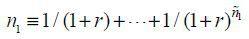 for the first stage, and
 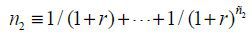 for the second. Note that multiplying
 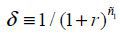 by n2 can provide fully discounted values based on the beginning of the first stage.
For a concise model, it is assumed that the generation levels of minor and stable sources are determined exogenously. Specifically, for stage t, let Xt denote the amount of annual pumping-up generation and heavy oil generation and Yt denote the renewable generation except for solar and wind power. The remaining energy sources can be divided into nonrenewable and renewable sources. Below, nonrenewable sources are represented by the subscript i, as follows: nuclear power (i = n), coal (i = c), and (liquefied natural) gas (i = l). Renewable sources are represented by subscript j, as follows: solar (j = s), and wind (j = w).
The RPS supply-obligation rate, applied to nonrenewable-based producers, is denoted by αt, and the price of a REC, endowed to renewable-based producers for 1 MWh of generation, is denoted by Bt. Depending on the energy source, REC weights are applied in consideration of policy factors (e.g., environment, technological development, and industrial activations; generation costs; potential capacities; GHG reduction effects; and power supply stability levels) in order to differentiate incentives depending on the source. The average REC weight, χj, is considered for both solar and wind power. The average weight for other renewable energy is set to 1.
Generation costs of producers can be divided into fixed costs (e.g., construction
costs, fixed operation maintenance costs) and variable costs (e.g., fuel costs, variable
operation maintenance costs). In South Korea’s wholesale market, the cost-based pool
is operated hourly by the Korea Power Exchange (KPX), where the system marginal price
(SMP),  is determined based on the variable costs of participating generators. To be specific,
in order to minimize the aggregate generation costs, participating generators are
ranked in the order of lower variable costs, and the last generator that meets the
forecast demand is defined as a marginal price generator. Because generators cannot
easily recover their fixed costs, the capacity payment (CP), φit, is additionally paid to all generators participating in the market. The Korea Electric
Power Corporation (KEPCO), a monopolistic distributer, purchases electricity by paying
various settlement amounts—capacity settlement amounts, energy settlement amounts,
RPS obligation compliance costs, and other charges—and supplies electricity to consumers
at the retail electricity price pt. By abstracting hourly decisions during a year, the model addresses the problem of
choosing annual generation levels at annual average prices.
is determined based on the variable costs of participating generators. To be specific,
in order to minimize the aggregate generation costs, participating generators are
ranked in the order of lower variable costs, and the last generator that meets the
forecast demand is defined as a marginal price generator. Because generators cannot
easily recover their fixed costs, the capacity payment (CP), φit, is additionally paid to all generators participating in the market. The Korea Electric
Power Corporation (KEPCO), a monopolistic distributer, purchases electricity by paying
various settlement amounts—capacity settlement amounts, energy settlement amounts,
RPS obligation compliance costs, and other charges—and supplies electricity to consumers
at the retail electricity price pt. By abstracting hourly decisions during a year, the model addresses the problem of
choosing annual generation levels at annual average prices.
A. Nonrenewable Generation
The generation of nonrenewable energy source i is denoted by xit, and its aggregate capacity is denoted by Kit. Let ζi denote the annualized construction cost for adding one unit (MW) of capacity for source i, taking its average lifespan into account. For each source at stage t, the wholesale settlement price according to the energy source is pit, which is a function of the SMP, as explained below. In addition, τi represents various policy charges levied on the amount of power generated by each nonrenewable energy source.
Under the assumed cost structure, for each energy source, the sum of individual firms’ cost functions is that of the representative firm, as is the profit. The cost function of the representative nonrenewable-based firm for source i at stage t is Ci(xit, Kit), which corresponds to the annual power generation costs (excluding construction costs) for generating xit.3 Suppressing subscripts for simplicity, it is assumed that cost functions satisfy Cx ≡ ∂C / ∂x > 0 and Cxx ≡ ∂2C / ∂x2 > 0 . That is, total costs and marginal costs increase in the generation amount. Further we assume CK < 0 and CKK > 0 . Therefore, total costs decrease in the capacity, while the marginal reduction of generation costs decrease in the capacity. By assuming CxK < 0 , we deal with situations where an additional capacity increase leads to a reduction in the marginal cost.
A representative nonrenewable energy firm has the follows profits:
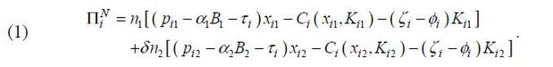
Equation (1) reflects the additional costs αtBt incurred to comply with the RPS obligation for one unit of nonrenewable generation. If a firm is simultaneously generating using nonrenewables and renewables, due to the separable cost structure, it can be understood that REC purchases and REC sales are occurring separately, where equation (1) only shows purchases.
In a competitive market, individual firms determine the amount of generation where the marginal cost curve (i.e., supply curve) matches the given price (e.g., Stoft, 2002; Borenstein and Holland, 2005; Biggar and Hesamzadeh, 2014). Given a linearly increasing individual supply curve, the slope becomes infinite (i.e., vertical marginal cost curve) after a firm’s generation reaches its maximum capacity. Thus, there are two situations: i) if the market price belongs to the vertical part of the supply curve, a firm generates to the maximum level of capacity, and ii) if the market price falls within the incremental part, it generates at the point where the price meets its supply curve. Note that the market price is determined at the point where the market-level supply curve and demand curve meet, where the annual market supply curve can be derived by horizontally summing individual marginal cost curves with respect to firms and hours.
The SMP in the wholesale electricity market is determined by the variable costs of a marginal generator. From an annual perspective, we consider that a representative gas-fired firm’s generation is determined at the point at which the aggregate marginal costs equal the wholesale settlement price under the given capacity.4 Assuming an interior solution, we exclude situations where the annual gas-fired generation becomes zero or reaches the maximum aggregate capacity. Then, for t = 1,2 and i = l equation (2) is established as a short-term equilibrium condition that determines the annual gas-fired generation.

On the other hand, we consider corner solution situations for nuclear and coal. The annual generation can be determined by multiplying the given capacity by the annual average capacity factor (βit) and by 8,760 hours (= 24 hours × 365 days). Therefore, for t = 1,2 and i = n, c, equation (3) holds as a short-term equilibrium condition.

In the long run, the generation capacity can increase or decrease freely. In the end, the long-run equilibrium condition is that the utility’s profit becomes zero (Borenstein and Holland, 2005). Therefore, over the long term, for t = 1,2 and i = n, c, l, equation (4) holds together with the short-term equilibrium conditions.

In the pricing structure of the domestic electricity market in South Korea, the settlement
price for nonrenewable energy, pit, is determined by an adjustment process based on the SMP (to maintain the financial
balance between KEPCO and its generation subsidiaries). Specifically, a typical settlement
price is calculated by 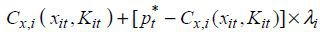 where is the SMP, Cx,i (xit, Kit) denotes the variable costs, and λi represents the adjustment coefficients. Furthermore, we consider that the per-MWh
compliance costs and various policy charges are also offset for producers, reflecting
the actual settlement process. Taking this feature into consideration, we have equation
(5) for t = 1,2 and i = n, c, l.
where is the SMP, Cx,i (xit, Kit) denotes the variable costs, and λi represents the adjustment coefficients. Furthermore, we consider that the per-MWh
compliance costs and various policy charges are also offset for producers, reflecting
the actual settlement process. Taking this feature into consideration, we have equation
(5) for t = 1,2 and i = n, c, l.

B. Renewable Generation
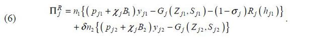
Following Fischer and Newell (2008) and Fischer, Preonas, and Newell (2017), we assume that the accumulative knowledge is Sjt = Sj(Hjt, Ljt). Note that Sjt is a function of knowledge from R&D, Hjt, and that from learning-by-doing, Ljt. We assume that SH > 0 and SL > 0 , as well as SHL = SLH. The annual new R&D knowledge generated in each stage, hjt, increases the cumulative R&D knowledge; i.e., Hj2 = Hj1 + n1hj1, and the annual production in each stage increases the accumulative experience knowledge; i.e., Lj2 = Lj1 + n1yj1. The R&D expenditure, Rj(hj1), is increasing and convex, i.e., Rh > 0 and Rhh > 0 , and R(0) = 0. The government supports proportion σj of renewable energy R&D expenditures.
When the above is reflected, profits for the representative renewable-based firm can be expressed as equation (6).
As mentioned above, the generation amount (MWh) is directly determined according to the capacity factor, and renewable generation satisfies equation (7).

With regard to knowledge accumulation, the degree of appropriability of newly acquired knowledge, ρ, can be considered, where we assume that solar power and wind power have the same value.5 Below, the incomplete transfer rate is considered (0<ρ<1), and for knowledge that a specific firm appropriates, other firms can use it by paying a license royalty. In particular, it is assumed that newly acquired knowledge is ultimately utilized through the use of either imitation or permission.6 As a result, the license revenue does not appear in equation (6), as this represents a simple transfer between firms.
The model takes into account second-stage cost savings which arise due to appropriable parts of new R&D-based knowledge in the first stage. Therefore, ρ appears in the representative firm’s first-order conditions, which are derived from those of the individual firms (see Appendix A. for the derivation). Finally, for j = s, w, the first-order condition associated with setting the value of the annual R&D knowledge, hjt, can be expressed as equation (8).

The first term in equation (8) is the amount of R&D net investment that must be paid in the first stage to acquire additional units of knowledge, and the negative of the second term represents discounted gains in the second stage from appropriating the new knowledge. Finally, the amount of new R&D knowledge is determined at the point where the cost and benefit are equal.
The long-term equilibrium condition of the representative renewable-based firm is to obtain a zero profit. This means that the excess profits from R&D investment are transferred to the consumers in the long run. For j = s, w, the long-term equilibrium condition is as follows:


In the case of renewable-energy sources, the SMP itself is the settlement price; thereby,
 .
.
C. Consumers
The electricity demand function is derived from the quasi-linear utility function of the representative consumer such that the consumer welfare can be consistently evaluated for each scenario in the simulation later. Specifically, the utility function can be expressed as U = I +Θ(P)−M. Here, I is the monetary income expressed by reference goods, and the price of the reference goods is normalized by 1. The demand function then becomes D(P) = −∂Θ / ∂P. For the sake of simplicity, peak demand during the year and resulting fluctuations in demand are not taken into consideration. In addition, it is assumed that the consumer considers environmental costs, M. Specifically, such costs apply to only coal and gas, which heavily emit GHG, and to the three major air pollutants NOX, SOX and PM2.5. Furthermore, it is assumed that consumers consider the possible nuclear accident costs (NAC), which are proportional to the capacity of nuclear plants. The five external costs above are expressed as εi,m, where m = GHG, NOX, SOX, PM2.5 for i = c, l and m = NAC for i = n. Finally, the total external cost can be expressed as Mt = Σi∈{c,l}Σm∈{GHG, NOX, SOX, PM2.5}εi,mxit + εn,ACKnt for t = 1,2 . Except for external costs, the consumer welfare for the two stages is expressed by equation (11).

The retail electricity price, Pt, is calculated by summing the aggregate settlement price,  , and the transmission and distribution costs per unit, Δ, and then adding the ad valorem sales tax ψ. As a result, for t = 1,2 equation (12) holds.

To be concrete, the aggregate settlement price, , is equal to the ‘total expenditure paid’ divided by the ‘total amount of electricity
purchased’ by the distributer in the wholesale market:
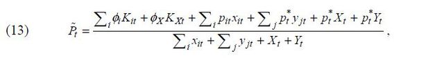
where φXKXt implies capacity charges for other nonrenewable energy sources.
In South Korea, although the discussion on price rationalization continues, the government regulates the retail electricity price, ensuring that it is not directly connected to the wholesale price. Under this circumstance, changes in the RPS obligation compliance costs cannot easily be fully reflected in the retail price. To examine the mid- and long-term market effects, however, in this paper we assume that the wholesale price is connected to the retail price in the future as well as in earlier periods.
D. Equilibrium
First, for t = 1,2 equilibrium in the power market must satisfy the equation

where ℓ is the loss ratio due to transmission and distribution.
Assuming full compliance under the RPS, the total amount of RECs, ∑jχjyjt + Yt, equals the obligation amount, αt×(∑ixit + Xt). As a result, the supply-obligation rate, αt, can be expressed as

Note that the numerator in equation (15) is based on effective units of renewable generation considering REC weights; accordingly, the physical amount of renewable generation decreases as the weights exceed 1, and vice versa. Later, we will look at the renewable share based on physical units, which is essentially related to achieving the policy goal.
Equilibrium in the integrated REC market requires that the demand and supply for RECs meet across renewable energy sources. In order to grasp the amount that a (marginal) buyer is willing to pay, equation (2) can be rewritten as

From the short-term standpoint of gas-fired firms, the left-hand side of equation (16) corresponds to the per-MWh gain that a gas-fired firm can earn in the wholesale market, and the right-hand side corresponds to per-MWh compliance costs. Regarding the long-term behavior, rearranging equation (4) yields the following expression for t = 1,2 and i = n, c, l,

where the left-hand side of equation (17) corresponds to the per-MWh gain in the long run. Note that for a gas-fired firm, it holds that Cx,i(xit, Kit) = [Ci(xit,Kit) + (ζi - φi)Kit] / xit from equations (16) and (17), indicating that for the marginal energy source, marginal costs equal average costs in the long run. Let the left-hand side of equation (17), identical for all i, be Φt. In a competitive integrated REC market, arbitrage cannot occur across energy sources. Thus, all nonrenewable-based firms pay Φt to comply with their per-MWh obligations.
For renewable sources, equations (9) and (10) can be rearranged as follows:


The left-hand sides of equations (18) and (19) correspond to the minimum acceptable amount for a REC seller, while the right-hand sides correspond to the REC sales revenue per 1MWh of renewable generation. In the competitive REC market, each left-hand side has a unique value regardless of the source, denoted by Ψt.
Using equations (17)-(19), for t = 1,2 REC market equilibrium can be defined as

Finally, equation (20) implies that the total compliance costs for nonrenewable generation and the total REC revenue for renewable generation are balanced. As long as the equilibrium REC price is greater than zero, the RPS imposes a burden on nonrenewable generation through the market mechanism and assists in the development of renewables. However, the burden of nonrenewables will eventually be passed on to consumers due to the compliance cost return mechanism, as explained in the context related to equation (13).
Under the RPS, equilibrium can be characterized by 34 equations from equations (2)-(5),
(7)-(10), (12), (14), and (20), which can be solved for 34 endogenous variables (xit, Kit, yjt, Zjt, ht, pit, , Pt, Bt for i = n, c, l, j = s, w, and t = 1,2 ). In order to analyze a situation without the RPS, equation (20) should be
dropped. Furthermore, in order to consider renewable energy subsidies, bjt, in the absence of the RPS, one can replace Bt with bjt in equations (9) and (10).
After finding the equilibrium values, the social welfare value can then be calculated. The consumer surplus, except for the externality costs, is equal to equation (11), and the external costs are equal to EX = n1M1 + δn2M2. The government net revenue is given by equation (21),
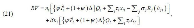
where Qt ≡ ∑ixit + ∑jyjt + Xt + Yt and is based on equation (13). Social welfare can be defined as W = PS + CS + RV + EX, where PS = 0 in the long run. This welfare measure has its limitations such that it ignores
benefits from enhancing national energy self-sufficiency or potential grid costs due
to the unstable characteristics of renewable energy sources. In the context of a lack
of related research in Korea, however, it still provides a useful metric of resulting
welfare effects caused by alternative renewable energy policies.
IV. Parameterization
To simulate the model, it is necessary to specify functions and set all parameters
in the model. In this section, based on raw data and information from the literature,
we set the parameter values by i) directly quoting raw data, ii) using the equilibrium
conditions in the model, or iii) introducing assumptions. In terms of the time horizon,
we set  in that it generally takes five years to obtain energy-related R&D results, and
  , having year 2030 positioned in the middle of the second stage. Roughly, five years
from 2015 to 2019, after the REC market is stabilized, can be regarded as the first
stage, and 20 years from 2020 to 2039 are considered as the second stage.7 Accordingly, the actual number of years in the first stage is n1 = 4.7, while that in the second stage is n2 = 10.6. The discount rate for the entire second stage is δ = 0.82. The energy market interest rate is assumed to be r = 0.07.8 As explained below, we use the raw data from 2016 for the first stage; thereby, all
monetary values are expressed in 2016 Korean won (₩). See the tables in Appendix B.
for a summary of values chosen in this section.
, having year 2030 positioned in the middle of the second stage. Roughly, five years
from 2015 to 2019, after the REC market is stabilized, can be regarded as the first
stage, and 20 years from 2020 to 2039 are considered as the second stage.7 Accordingly, the actual number of years in the first stage is n1 = 4.7, while that in the second stage is n2 = 10.6. The discount rate for the entire second stage is δ = 0.82. The energy market interest rate is assumed to be r = 0.07.8 As explained below, we use the raw data from 2016 for the first stage; thereby, all
monetary values are expressed in 2016 Korean won (₩). See the tables in Appendix B.
for a summary of values chosen in this section.
A. Primary Data
Information about capacity, generation, and price levels in the first stage are based on 2016 data from KEPCO (2017). For the second stage, we use projected values for the year 2030 provided by MOTIE (2017), reflecting RE3020. Other nonrenewable energy generation, Xt, is assumed to be fixed over the first and second stages; these values are calculated using the 2016 raw data of KEPCO (2017). For other renewable energy generation, Y1 is based on KEPCO’s (2017) raw data, while Y2 is constructed using projected values from MOTIE (2017), reflecting an increasing trend of the other renewable category. For the amount of electricity that is actually supplied in the wholesale market, based on KPX (2018), intra-plant load factors, ωi, are considered for nonrenewable sources though not for renewable sources.
Figures regarding R&D spending on core renewable technologies is collected from internal
data of Korea Energy Technology Evaluation and Planning (KETEP). Cumulative R&D knowledge
of solar power in the first stage is normalized as Hs1 =1, and cumulative knowledge of wind power is calculated as Hw1 = 0.69 by considering the proportion of relative R&D expenditures during 2007-2016.
Cumulative experience knowledge, Lj1, is estimated using cumulative generation volumes during 2005-2016. The amount of
new R&D knowledge obtained through the first stage, hj1, can be calculated using equation (9), which requires information about second-stage
generation. Therefore, we start with the projected 2030 capacity values to calculate
 and then input in equation (9) to obtain the estimated capacity values. Iterating this procedure
until precisely replicating the first stage value can give us the reference value
of hj1.
and then input in equation (9) to obtain the estimated capacity values. Iterating this procedure
until precisely replicating the first stage value can give us the reference value
of hj1.
Hourly CP rates for nonrenewable sources are derived using internal data of the KPX, and corresponding annual rates are calculated by considering plant utilization factors (KPX, 2014). Annualized fixed costs for nonrenewable and renewable energy sources come from KPX (2018)’s data, which are similar to ‘overnight costs divided by the plant lifetime’ based on figures from the International Energy Agency (IEA) and Nuclear Energy Agency (NEA) (2015). Retail costs are calculated using KEPCO’s Electricity Cost Information for 2013-2017. Specifically, the total sales figure of the retail market minus the cost of purchasing electricity is regarded as the residual retail cost, which is ₩19,355/MWh. The degree of appropriability is set to 0.5 for both solar power and wind power in keeping with Fischer, Preonas, and Newell (2017), meaning that the social return of R&D is double the private return.
B. Functional Assumptions
For nonrenewable sources i = n, c, l, we employ quadratic cost functions that satisfy foregoing assumptions,  , where the superscript BL indicates baseline values. Because
  , we can calibrate c0,i, which corresponds to all fixed costs except for the annualized construction costs,
based on equation (4). Given the above cost functions, marginal cost functions are
, we can calibrate c0,i, which corresponds to all fixed costs except for the annualized construction costs,
based on equation (4). Given the above cost functions, marginal cost functions are
 , and at the baseline
  . First, one can obtain c1, l, which corresponds to gas power marginal costs at the baseline, using equation (2).
Based on the internal data of KPX, we horizontally sum individual marginal cost functions
to obtain aggregate marginal cost functions according to the energy type and derive
c1,i for i = n, c and c2,i for i = n, c, l.
. First, one can obtain c1, l, which corresponds to gas power marginal costs at the baseline, using equation (2).
Based on the internal data of KPX, we horizontally sum individual marginal cost functions
to obtain aggregate marginal cost functions according to the energy type and derive
c1,i for i = n, c and c2,i for i = n, c, l.
Cost functions for renewable sources j=s,w are specified as  , where g0,j captures fixed costs apart from annualized construction costs. One can calibrate
g0,j using equation (9). For j=s,w, knowledge functions are Sj(Hjt, Ljt) = (Hjt / Hj1)s1,j(Ljt / Lj1)s2,j, where the cumulative knowledge stock has constant elasticity with respect to R&D
knowledge and experience knowledge, and the first-stage knowledge stock is normalized
to 1, i.e., Sj(Hj1, Lj1) = 1 . R&D knowledge parameters are set to s1,s = s1,w = 0.3 and learning knowledge parameters are set to s2,s = s2,w = 0.3; thus, projected outcomes under RE3020 are roughly implemented in the baseline.
R&D expenditure functions are
, where g0,j captures fixed costs apart from annualized construction costs. One can calibrate
g0,j using equation (9). For j=s,w, knowledge functions are Sj(Hjt, Ljt) = (Hjt / Hj1)s1,j(Ljt / Lj1)s2,j, where the cumulative knowledge stock has constant elasticity with respect to R&D
knowledge and experience knowledge, and the first-stage knowledge stock is normalized
to 1, i.e., Sj(Hj1, Lj1) = 1 . R&D knowledge parameters are set to s1,s = s1,w = 0.3 and learning knowledge parameters are set to s2,s = s2,w = 0.3; thus, projected outcomes under RE3020 are roughly implemented in the baseline.
R&D expenditure functions are  for j = s, w, which yield constant elasticities, γ2,j. Following Fischer and Newell (2008) and Fischer, Preonas, and Newell (2017), we set γ2,j = 1.2 for j=s,w,9 with γ1,j calculated using equation (8).
A constant elasticity aggregate demand function is utilized, in this case D(Pt, Nt) = Nt × (Pt)η, where the price elasticity of electricity demand, η, is assumed to be -0.3 from a mid- to long-term perspective. Several recent domestic studies estimate the elasticities of electricity demand as follows. Kim and Park (2013), using monthly consumption data for 1981-2011, suggest that the price elasticity rates of industrial (residential) consumption are -0.127 (0.143) before 1997 and -0.088 (0.123) after 1997. Lim, Lim, and Yoo (2013), based on survey data of 521 households in 2012, estimate the price elasticity of residential consumption as - 0.68. As examples of elasticity application for a model simulation, Borenstein and Holland (2005) assume that the demand elasticity is -0.1 in the short run and -0.3 or -0.5 in the long run. In Fischer and Newell (2008), it is assumed to be -0.2 from a long-term perspective, while Fischer, Preonas, and Newell (2017) apply -0.1 from a short-term perspective. Note that Nt represents exogenous changes in the power demand level. We apply N1 = 1.64 × 10¹⁰ considering the baseline price and quantity and N2 = 1.85×10¹⁰ (= N1 × 1.125) based on MOTIE’s (2017) projected increase in demand.
The solar and wind capacity factors in the first stage are calculated as βs1 = 0.138 and βw1 = 0.182, respectively, using aggregate generation and capacity data from KEPCO (2017). For the second stage, βs2 = 0.14 which is the average of the predicted capacity factor values for 2017-2031. We also set βw2 = 0.21 by assuming that the wind capacity factor increases at a rate identical to that of the solar power.
C. Externality Costs
GHG social costs in the first stage are assumed using Yi’s (2018) results, which are the basis of the recently published Financial Reform Special Committee (2018): ₩35,680/MWh for coal and ₩15,720/MWh for gas. When referring to figures in old publications—emission factors in MOTIE (2014) and marginal damages in MOTIE (2015)—we have externality costs of ₩20,575/MWh for coal and ₩9,063/MWh for gas. Accordingly, it appears that external costs are experiencing upward adjustments to reflect increasing environmental damages.
With respect to GHG externality costs in the second stage, an additional discussion regarding the trends of the estimates in the literature is necessary. The US Government (2016) specifies that under three discount rate assumptions (5%, 3%, and 2.5%), the US CO2 social costs in 2030 compared to 2015 are greatly increased (46%, 39%, and 30%). Nordhaus (2017), relying on the updated Dynamic Integrated Model of Climate and the Economy (DICE), presents estimates of the global CO2 social cost of $31.2/tCO2 in 2015 and $51.6/tCO2 in 2030, indicating an increase of 65%. In addition, applying the discount rate of Stern (2007), which is approximately 1.4%, the corresponding values are estimated to be $197.4/tCO2 in 2015 and $376.2/tCO2 in 2030, resulting in an increase of 91%. Along with the trends in these estimates, we assume that the discounted GHG social costs in the second stage are 34% higher than those in the first stage, applying a discount rate of 7%; these outcomes are ₩47,759/MWh for coal and ₩21,042/MWh for gas. Thereby, we specify costs as εit,GHG for i = n, c and t = 1, 2.
Air pollutant social costs follow the values given by Yi (2018): NOX, SOX and PM2.5, respectively, cause social costs of ₩16,590/MWh, ₩15,740/MWh, and ₩800/MWh for coal, and ₩4,630/MWh, ₩310/MWh, and ₩320/MWh for gas. These figures are applied in both stages without trends because air pollutants cause damages locally and do not stay in the atmosphere for a long time. In addition, the nuclear accident risk cost is based on the value provided by KPX (2018), where several alternatives are specified depending on how the probability of an accident is handled. We employ the estimate of ₩67,644,000/MW, as finally determined in the analysis by KPX (2018).
V. Numerical Simulation
A numerical simulation is carried out for six policy scenarios: i) the baseline RPS, ii) repealing the RPS, iii) the past RPS, iv) the optimal RPS, v) a renewable generation subsidy, and vi) nuclear power reduction. The baseline RPS scenario presents market outcomes under the 2016 RPS in the first stage and under the implementation of RE3020 (i.e., 20% share of business-purpose renewable generation) in the second stage. Renewable generation occupies 5.0% in the first stage and 20% in the second stage, where the corresponding RPS supply-obligation rates are 5.5% and 28%, respectively. In this scenario, while the supply-obligation rate determines the amount of renewable generation, the market drives the amount of generation for the remaining energy sources, where the wholesale and retail prices remain connected for both stages.
The repeal of the RPS scenario deals with a situation in which only the RPS is removed, where we assume that a certain level of renewable energy (mostly hydro) continues.10 Compared to the baseline, the past RPS scenario is based on the second-stage supply-obligation rate as stipulated before RE3020. Specifically, it was to apply 4% in 2017 and, by increasing by 1% each year, reach 10% in 2023. Reflecting this trend, we apply 17% in 2030. In the optimal RPS scenario, the second-stage supply-obligation rate is set such that it maximizes the social welfare, while we hold the first-stage rate at the same level.
The subsidy scenario, in the absence of the RPS, introduces a direct production subsidy for renewable generation. To compare with the baseline, the subsidy level is set precisely using the REC prices for each stage in the baseline, i.e., ₩98,807/MWh and ₩5,781/MWh, respectively. The nuclear reduction scenario forces a 5% reduction in the aggregate nuclear power capacity in the second stage compared to the baseline, maintaining the same capacity factor.11
Equilibrium outcomes for each scenario can be obtained by solving the calibrated model based on corresponding sets of equilibrium conditions and assumed policy parameters. The welfare effects, aggregated over both stages, refer to relative welfare changes compared to the scenario without the RPS. As a result of the simulation, the market results for each scenario are as shown in Table 2 and the welfare effects are as shown in Table 3. When the parameters were set correctly, the first-stage baseline outcomes are consistent with the figures from primary data. It turns out that the first-stage market results are consistent with the raw data.
TABLE 2
SIMULATION RESULTS: MARKET OUTCOME
Note: All scenarios except for the no RPS scenario are under government R&D support.
TABLE 3
SIMULATION RESULTS: WELFARE OUTCOME (₩ BILLION)
Note: Welfare effects are changes relative to the no RPS scenario.
A. Baseline RPS and Repeal of the RPS
In the baseline scenario, the first-stage market results replicate the raw data, while the second-stage results are of interest because there are no values to be replicated other than the renewable generation capacity. It was found that if an RPS supply-obligation rate of 28% is applied in the second stage, the renewable share increases to 19.6%, where the annual solar and wind power generation levels are similar to each other. Specifically, the annual generation levels are 32,544 MWh for solar and 46,627 MWh for wind. This is quite similar to the plans for these two power sources (33,530MWh for solar and 42,566MWh for wind) by MOTIE (2017).
In the baseline, the annual R&D expenditure in the first stage is approximately ₩87.1 billion/year for solar (₩435.5 billion in total during the first stage) and about ₩70.1 billion/year for wind (₩350.5 billion in total). Compared to the first stage, in the second stage the generation costs are reduced by 24.7% for solar and 17.3% for wind, owing to technology development and learning effects. Under the cost reduction, the REC price drops to ₩5,781/REC but remains positive, meaning that the RPS is binding even in the second stage. In other words, generation costs for renewable energy are still higher than the costs for fossil fuels.
The second-stage retail price fell by 4.1% from that in the first stage due mainly to a decline in the generation costs for renewable energy. Owing to the reduced REC price, the annual RPS compliance cost (= REC price×weighted renewable energy generation) dropped greatly from ₩2.7 trillion/year in the first stage to ₩76 billion/year in the second stage. In addition, due to the expansion of renewable energy, the generation volume of nonrenewable energy in the second stage is reduced compared to that in the first stage. The generation mix consists of 30% nuclear, 39% coal, 23% gas, 3% other nonrenewables, and 5% renewable in the first stage, and with corresponding rates of 26%, 35%, 17%, 3% and 20% in the second stage. The resulting capacity factors for nuclear, coal and gas are 76%, 73%, and 42% in the first stage and 76%, 73%, and 35% in the second stage, respectively, where there is a decrease only in gas-fired generation. The reduced generation volume contributes to lower nonrenewable-energy marginal costs, resulting in a slight decline of 0.03% in the wholesale electricity price. As a result of this price effect, annual electricity consumption in the second stage is increased by 13.9% from the first stage, which exceeds the exogenous demand increase of 12.5%.
When the RPS is abolished, there is no renewable generation in either the first or second stages, and no R&D investment in renewable energy occurs. The wholesale settlement price rises slightly by 0.11% from the first stage to the second because marginal costs increase as nonrenewable generation increases due to the increase in exogenous demand. The retail price declines by 0.5% in the second stage compared to the first stage because there is a decrease in capacity payments in the second stage, which overwhelms the increase in the wholesale settlement price. Compared to the repeal of RPS scenario, in the baseline scenario retail prices are increased by 5.0% in the first stage and 1.1% in the second stage. In other words, under the RPS, it can be understood that the payment for the RPS compliance cost is placed on top of the wholesale adjusted price, causing an increase in retail prices. As a result, total consumption in the baseline scenario is decreased by 1.4% in the first stage and 0.3% in the second stage, relative to the no RPS scenario.
With regard to welfare effects, the baseline scenario, compared to the no RPS scenario, shows a welfare increase of ₩44.7 trillion, which means a relative gap in the discounted 25-year welfare sum. Looking at distributional effects, government revenue in the baseline is reduced compared to the no RPS scenario mainly due to i) an additional R&D expenditure and ii) lower wholesale tax revenue. Compared to the no RPS scenario, in the baseline increased retail prices lower consumer surplus by ₩18.5 trillion, while the reduced amount of nonrenewable generation results in lower externality costs of ₩63.6 trillion.
B. Past RPS and Optimal RPS
In terms of the second-stage supply-obligation rate, which is 28% in the baseline, the past RPS and optimal RPS scenarios respectively apply a lower rate of 17% and a higher rate of 31%. Note that as the second-stage rate increases, i.e., when we go through ‘no RPS’ → ‘past RPS’ → ‘baseline RPS’ → ‘optimal RPS’, the second-stage wholesale price decreases. This occurs due to the merit-order effect, by which a decrease in nonrenewable energy generation due to the strengthening of the RPS results in lower marginal costs at the margin. On the other hand, first-stage retail prices increase as the RPS is strengthened because a stronger second-stage supply-obligation rate necessitates a larger expansion of wind power, which is more expensive than solar power, thereby leading to rises in the REC price and retail price in the first stage.
It is important to examine changes in R&D investments. First, as the second-stage supply-obligation rate increases, the annual R&D investment increases significantly for both solar and wind power. This arises because if second-stage renewable generation is forcibly increased, the R&D incentive becomes stronger because the marginal effects of the second-stage cost reduction from the first stage of R&D increases. It appears that as the second-stage supply-obligation rate increases, the greater cost-reduction effects realizes. In addition, strengthening the RPS results in a larger role of wind power; thereby, wind power experiences a greater cost reduction from the baseline than solar power in the optimal RPS scenario. This arises because the first-stage accumulative knowledge stock for wind is lower than that of solar, meaning that the marginal cost-reduction effects from additional knowledge is higher for wind than for solar.
In term of welfare, when normalizing the welfare increase from the no RPS scenario to the past RPS scenario as 1, the baseline undergoes an increase in welfare by 1.7 times and the optimal RPS scenario experiences an increase by 1.9 times. In detail, the stronger the RPS supply-obligation rate is in the second stage, the higher the incentive for R&D investment becomes, resulting in higher government expenditures. A stronger second-stage supply-obligation rate also lowers consumer surplus with an increase in retail prices. Despite these negative effects, overall welfare increases in the second-stage RPS target rate owing to the considerable decrease in externality costs.
C. Renewable Generation Subsidy and Nuclear Power Reduction
In the subsidy scenario, it turns out that when subsidy levels are precisely equal to REC prices, the resulting renewable energy generation and cost saving effects are identical to those in the baseline scenario. As the RPS obligation is not incurred, however, retail electricity price falls by 4.8% in the first stage and by 1.2% in the second stage compared to the baseline scenario. Wholesale prices are higher in the subsidy scenario because nonrenewable energy generation is greater, yielding higher marginal costs than in the baseline.
As a result, replacing the RPS with a renewable generation subsidy yields a gain of ₩19.1 trillion in consumer surplus compared to the baseline, as electricity is supplied at lower retail prices. On the other hand, compared to the baseline, there is an increase in the government expenditure of ₩19.3 trillion, and the amount of nonrenewable energy generation increases, resulting in reduced external costs of ₩1.8 trillion. In summary, the effect of raising overall welfare from the no RPS scenario is ₩2.6 trillion lower than that in the baseline scenario.
As shown in Table 2, an introduction of the RPS from its absence mainly reduces gas-fired generation, which is marginal in terms of generation, and has minor effects on the remaining nonrenewable energy sources. In the baseline scenario, the second-stage nuclear power capacity is determined to be approximately 23,124MW, and nuclear generation accounts for 26.0% of the total in the second stage. The nuclear reduction scenario is to, from the baseline, limit aggregate nuclear capacity to 21,968 MW, which is a 5% reduction, thereby reducing nuclear generation from 153 TWh to 146 TWh under the baseline nuclear capacity factor, accounting for 24.6% of the total generation.
The forced reduction in the second-stage aggregate nuclear capacity results in an increase in the retail price owing to the increases in other expensive forms of nonrenewable generation. As a result, compared to the baseline, consumer surplus is lowered by about ₩300 billion, and producer surplus in nuclear power experiences a loss of ₩3.6 trillion as the long-term equilibrium condition is not met with increased marginal costs. The costs associated with the nuclear accident risk are reduced by about ₩640 billion compared to the baseline scenario, but the environment external costs are more than ₩3.2 trillion due mainly to the increased amount of gas-fired generation. As a result, overall welfare is lower by ₩7.9 trillion than in the baseline.
The nuclear power reduction scenario can be thought of as a further reflection of MOTIE (2017) when considering the schedule of nuclear power capacity. One can also interpret the result of this scenario in the following way. When setting the nuclear power reduction scenario as the baseline, the original baseline scenario can be treated as a scenario in which market principles are applied to the nuclear power sector ceteris paribus. The implication is then as follows: if letting the market mechanism fully govern the nuclear power sector, there would be welfare gains partially from an increase in nuclear power generation and a decrease in gas-fired generation. This outcome mainly arises because nuclear power generation is less expensive than generation by other energy sources, resulting in overall welfare gains even if considering the negative impacts from nuclear accident risks.
D. Sensitivity Analysis
A sensitivity analysis is performed while changing major parameter values. Table 4 summarizes the variations of the parameters and the resulting welfare effects. To be specific, the analysis deals with changes in the discount rate, the length of the second stage, the level of demand elasticity, the R&D effect, the learning effect, and the appropriability rate, while also removing exogenous demand growth, second-stage efficiency improvements, and any increase in the second-stage GHG social costs, with 15 cases analyzed in total. It should be noted that the relative welfare rank among the six scenarios remains the same throughout the analysis. Specifically, from the highest welfare scenario, the order is as follows: optimal RPS, baseline RPS, renewable generation subsidy, nuclear reduction, past RPS, and repeal of RPS, where the magnitude of the welfare effect continues to vary.
TABLE 4
SENSITIVITY ANALYSIS
Note: 1) Welfare effects are changes relative to the no RPS scenario. 2) In the case of ‘low GHG social costs’, it is assumed that the second-stage discounted GHG costs of coal and gas are identical to those in the first stage.
There are several notable features. If we increase the discount rate from 7% to 9%, the present value of future benefits and costs become smaller; thus, the overall welfare effect gap between the scenarios is reduced compared to that in the baseline. On the other hand, if the discount rate is reduced to 5%, the relative gap becomes larger than in the baseline results. Note that reducing or increasing the number of years in the second stage has the same effect as raising or lowering the discount rate applied to the second stage, thereby yielding similar results compared to an adjustment of the discount rate.
Lowering the demand elasticity reduces the magnitude of the overall welfare effects for all scenarios, while increasing it results in larger welfare changes, where for the latter demand responses are more significant. The changes in welfare by varying the R&D effect, learning effect, and appropriability are lower compared to the former variations. The elimination of the natural demand growth in the second stage compared to the first lowers welfare for all scenarios, and removing the improvement in the renewable capacity factor also results in lower welfare. When assuming that the discounted second-stage GHG social costs are maintained at the level of the first stage, the magnitude of the welfare effects is lower than in the baseline for all scenarios.
VI. Concluding Remarks
This paper analyzes the market and welfare effects of South Korea’s policy goal, RE3020—raising the proportion of renewable energy generation to more than 20% by 2030—together with other policy options. To carry out counterfactual simulations for alternative scenarios, we propose a model that reflects the major characteristics of the domestic electricity market. In particular, the model incorporates the energy settlement system in the wholesale electricity market and REC transactions under the RPS, as well as R&D investment and learning effects that may affect the development of renewable energy technologies. The model consists of a first stage in which knowledge related to renewable energy technology development accumulates and a second stage in which technology development is realized due to accumulated knowledge. As a reference scenario for the simulations, the first and second stage in the model are parameterized to replicate the current situation (based on raw data in 2016) and the future that reflects the implementation of RE3020 (based on projected values over 2017-2031), respectively. Subsequently, we simulate alternative scenarios to investigate the relative performance outcomes among them.
The results show that the current and planned RPS under RE3020, which is set as a baseline, increases social welfare compared to the weakened RPS before RE3020, and compared to the absence of the RPS. Although introducing or reinforcing the RPS causes an increase in retail electricity prices, hurting consumers, it crowd out nonrenewable energy generation owing to the merit order effect, thereby resulting in a significant reduction of externality costs. As long as it is feasible in terms of the physical area, it is found that welfare can be increased further by strengthening the RPS beyond what RE3020 stipulates. As an alternative to the RPS, a simple production subsidy for renewable energy is examined, and it turns out that welfare is lower than the RPS when the same level of renewable energy generation is achieved. This occurs mainly because the government must incur a major financial burden. Finally, restraining nuclear power generation from the baseline is found to lower welfare compared to the baseline because an increase in externality costs from expanded coal and gas power generation overwhelms the decrease in nuclear accident costs.
The Paris Agreement was signed at the 21st Conference of the Parties of the UNFCCC in 2015 on the basis of a global consensus on countering climate change and improving energy self-sufficiency. Since then, energy conservation has been promoted worldwide by expanding renewable energy, improving production efficiency, and saving energy. As a result of the Paris Agreement, South Korea is expected to achieve a GHG emission reduction of 37% relative to ‘business as usual’ by 2030, where one of the measures proposed is the use of the RPS in the power sector. In this context, the analysis in this study attempts to present a measure of the impact of South Korea’s major renewable energy policy, the RPS.
However, there are several caveats to consider when interpreting the results in this paper. When the generation share of variable renewable energy sources exceeds a certain level, the power grid system may undergo daily weather fluctuations when attempting to maintain a stable supply. To illustrate this, in locations where a significant amount of solar power capacity has been installed, the amount of power that must be generated from sources other than solar energy increases sharply around sunset. Then, the grid system would require additional costs by preparing back-up generation and/or large-scale energy storage systems, factors which are not taken into account in this paper. Depending on the levels of the related costs and who pays such a burden, the results can be affected. In addition, the analysis is based on the assumption that all electricity market policies except for those we are tackling will remain identical to those in the current situation. Finally, this paper does not consider possible electricity demand management scenarios or incentives for residential selfgeneration.
Appendices
APPENDIX
A. Derivation of Equation (8)
Applying Fischer and Newell’s (2007) framework, we derive ρ in equation (8) from individual firms’ first-order conditions, given that some innovations
of a particular firm may be appropriable. For j = s, w, suppose that there are Nj identical firms, and let the subscript k denote an individual firm. Assume that the cumulative knowledge is completely disseminated,
yielding 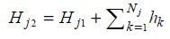 and
and 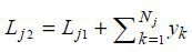 . A share of ρj for R&D knowledge cannot be imitated and can be used by paying a license fee. We
then have the following individual firm k ’s profit,
. A share of ρj for R&D knowledge cannot be imitated and can be used by paying a license fee. We
then have the following individual firm k ’s profit,
where 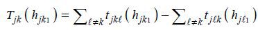 . Note that Tjk(hjk1) denotes loyalty income from other firms, netting payments to other firms. To be
specific,
. Note that Tjk(hjk1) denotes loyalty income from other firms, netting payments to other firms. To be
specific,  , meaning that the (maximum) loyalty that a firm k can collect from a firm ℓ is the amount of cost savings that firm ℓ can achieve by accessing firm k ’s knowledge that cannot be imitated.
When all licenses are fully accessed under a symmetric equilibrium, the marginal loyalty gain from a unit of innovation is as follows:
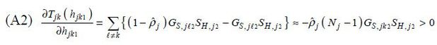
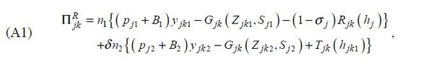
If a firm k increases its R&D-based knowledge by one more unit, there will be more room for second-stage cost reductions (whether through imitation or licensing) for other firms. Here, due to ρj, the marginal cost reduction by using full licenses is greater than that by simply imitating. Hence, when firm k generates one more unit of innovation, other firms consider paying royalty more beneficial compared to imitating. Meanwhile, the choice of firm k to use other firms’ licenses is not affected by its innovation choice. Therefore, an increase in R&D knowledge increases loyalty income, as expressed by equation (A2). Considering this feature, we have the following first-order condition for an individual firm’s innovation choice.

Royalty payments refer to a simple transfer between firms: ∑kTjk(hjk1) = 0. Under symmetric equilibrium by energy sources, we have yjt = ∑kyjkt, Zjt = ∑kZjkt, hjt = ∑khjkt, and Gj(Zjt, Sjt) = ∑kGjk(Zjt, Sjt). Because accumulative knowledge is shared by all firms, we have ∂G(Zjt, Sjt) / ∂Sjt = Nj∂Gjk(Zjkt, Sjt) / ∂Sjt. Moreover, total R&D spending is the sum of individual firms’ R&D spending; i.e., Rj(hj1) = ∑kRjk(hjk1). Thus, Rh,j(hj1) = Rh,jk(hjk1).
Based on the conditions above, we have  first and then obtain the following by aggregating equation (A3).

Here, 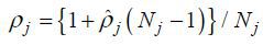 , and as Nj becomes larger, ρj approaches
  . For simplicity, we can assume ρs = ρw = ρ, which makes equation (A3) equal to equation (8).
B. Tables
TABLE A1
RAW AND PROCESSED DATA
Note: The superscript BL indicates values replicated from the baseline scenario. Other renewable generation includes generation from some nonrenewable waste and new energy sources which are projected to be fairly stable according to MOTIE (2017).
Notes
This paper is based on Kim, Hyunseok, 2018, “Welfare Impacts of the Renewable Portfolio Standard in Korea,” Policy Study 2018-17, KDI (in Korean). Special thanks are due to Minhye Choi for her devoted research assistance and to KPX and KETEP for providing raw data related to the wholesale electricity market. Valuable comments by two anonymous referees are appreciated.
Following the Implementation Plan for RE3020, the definition of renewable energy in this paper includes some nonrenewable waste (e.g., industrial waste and nonrenewable urban waste) and new energy sources (e.g., fuel cells), which play a small role in the plan. Meanwhile, the International Energy Agency’s (IEA) definition of renewable energy only includes hydropower, geothermal, solar, wind, tidal and bioenergy sources, excluding nonrenewable waste and new energy sources (IEA, 2002). Based on the IEA definition, South Korea’s share of renewable energy in 2016 was 2.8% (IEA, 2018a).
In South Korea, every two years MOTIE establishes the Basic Plan for Long-Term Electricity Supply and Demand, setting a schedule for generation capacity. This plan is actually based upon survey results regarding construction and abolishment intentions in the private sector in order to reflect the long-term market reaction to the plan. Therefore, an analysis regarding long-term market equilibria can be a useful criterion in terms of approximating market results under possible national plans.
Note that xit is the amount of electricity sold to the wholesale electricity market after subtracting plants’ intra-consumption amounts, and this value is used as the basis for calculating the obligatory supply under the RPS.
According to SMP determination data by fuel source from the Electric Power Statistics Information System (EPSIS) (http://epsis.kpx.or.kr/epsisnew/selectEkmaSmpNsmGrid.do?menuId=050203, accessed Aug. 31, 2018), the fuel-type shares of marginal generators for 2010-2017 are 87% for gas (LNG), 9% for oil, and 4% for coal. We abstract daily demand fluctuations and consider gas-fired plants as marginal on an annual basis.
For example, ρ=0 implies that the newly acquired knowledge of an individual firm is completely spilled over to other firms, while ρ=1 implies that new knowledge is fully attributed to the corresponding firms.
Qiu and Anadon (2012) attempt empirically to identify the impact of expanding wind power on the decline in China’s electricity prices during the period of 2003-2007 (without distinguishing between R&D innovations and learning effects), finding that knowledge spillover among firms has contributed significantly to the decline. The authors rationalize the results considering that both the government and business operators are gaining information about management and operation during the expansion of the industry.
Regarding the length of the stage required for innovation, Newell, Jaffe, and Stavins (1999) consider that the energy efficiency enhancement of household appliances is up to five years. On the other hand, EIA (2011) and EIA (2014) establish typical cost recovery periods for power generation technology of 18 years and 28 years, respectively. Practically, Fischer and Newell (2008) and Fischer, Preonas, and Newell (2017) assume five years for their first stages and 20-21 years for their second stages.
In IEA and NEA (2015), a discount rate of 7% is applied as a median value for calculating the levelized cost of energy for each country. In addition, IEA (2018b) has recently stated that the energy industry’s market interest rate remains stable at around 6%.
The elasticity of patent R&D is estimated to be 0.8 by Jaffe (1986); based on the reciprocal of the estimate, Fischer and Newell (2008) calculate the elasticity of new knowledge of R&D as 1.2.
An average renewable generation level of 102,150 MWh for 1999-2000, which was before the introduction of the FIT, is regarded as the minimum amount of renewable energy generation.
As shown later, in the baseline, the second-stage aggregate nuclear capacity is 23,024 MW. On the other hand, MOTIE (2017) forecasts that the nuclear capacity will increase from 22,529 MW in 2017 to 28,200 MW in 2023 and then decline to 20,400 MW in 2029. In order partially to reflect the capacity projections around 2030 in MOTIE (2017), which appears to be based on the government’s plan, the scenario of ‘nuclear power reduction’ artificially reduces the aggregate nuclear capacity from the baseline.
References
, , & . (2017). Market and Welfare Effects of Renewable Portfolio Standards in United States Electricity Markets. Energy Economics, 64, 384-401, https://doi.org/10.1016/j.eneco.2017.03.011.
, , , & . (2014). Alternative Transportation Fuel Standards: Welfare Effects and Climate Benefits. Journal of Environmental Economics and Management, 67(3), 241-257, https://doi.org/10.1016/j.jeem.2013.09.006.
Electric Power Statistics Information System (EPSIS). Electric Power Statistics Information System (EPSIS), http://epsis.kpx.or.kr/epsisnew/selectEkmaSmpNsmGrid.do?menuId=050203, accessed Aug. 31, 2018.
, & (2008). Environmental and Technology Policies for Climate Mitigation. Journal of Environmental Economics and Management, 55(2), 142-162, https://doi.org/10.1016/j.jeem.2007.11.001.
, , & (2017). Environmental and Technology Policy Options in the Electricity Sector: Are We Deploying Too Many? Journal of the Association of Environmental and Resource Economists, 4(4), 959-984, https://doi.org/10.1086/692507.
, & . (2013). Changes in Elasticities of Demand for Oil Products and Electricity in Korea. Environmental and Resource Economics Review, 22(2), 251-279, in Korean, https://doi.org/10.15266/KEREA.2013.22.2.251.
Korea Energy Agency, New and Renewable Energy Center. Korea Energy Agency, New and Renewable Energy Center, New and Renewable Energy Supply Statistics, https://www.knrec.or.kr/pds/statistics.aspx, accessed Nov 19, 2018.
(2007). Impacts of a Renewable Portfolio Generation Standard on US Energy Markets. Energy Policy, 35(2), 809-814, https://doi.org/10.1016/j.enpol.2006.03.002.
, , & . (2013). Estimation of Residential Electricity Demand Function Using Cross-Section Data. Journal of Energy Engineering, 22(1), 1-7, in Korean, https://doi.org/10.5855/ENERGY.2013.22.1.001.
, , & . (2017). The Renewable Fuel Standard in Competitive Equilibrium: Market and Welfare Effects. American Journal of Agricultural Economics, 99(5), 1117-1142, https://doi.org/10.1093/ajae/aax041.
, , & (1999). The Induced Innovation Hypothesis and Energy-Saving Technological Change. Quarterly Journal of Economics, 114(3), 941-975, https://doi.org/10.1162/003355399556188.
, & (2005). Does Britain or the United States Have the Right Gasoline Tax? American Economic Review, 95(4), 1276-1289, https://doi.org/10.1257/0002828054825510.
, & (2012). The Price of Wind Power in China during its Expansion: Technology Adoption, Learning-by-Doing, Economies of Scale, and Manufacturing Localization. Energy Economics, 34(3), 772-785, https://doi.org/10.1016/j.eneco.2011.06.008.
U.S. Government. (2016). Technical Support Document: Technical Update of the Social Cost of Carbon for Regulatory Impact Analysis under Executive Order 12866. Technical Support Document: Technical Update of the Social Cost of Carbon for Regulatory Impact Analysis under Executive Order 12866. Interagency Working Group on Social Cost of Greenhouse Gases.