Equity across Generations and Uncertainty within a Generation: A Welfare Analysis of the National Pension System^†

A. Demographic Structure

Time t is discrete and the model period is one year. The model economy is populated by J_D overlapping generations. Individual workers may live up to J_D periods and face mortality risks in each period. Let ψ_T( j,t) denote the conditional probability that an individual of age j in period t survives to the next period t + 1. Let n_T(t) denote the growth rate of the population of age 1 in period t . Let N_j,t(1 ≤ j ≤ J_D denote the population of age j in period t . The total population in period t is calculated as .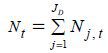

Then, the population of each age evolves over time, as follows:

We refer to the population of age j in period t as the k_th cohort. Note that age, time, and cohort indices are not independent given the one-to-one function that k = t − j + 1 . In order to simplify the notations and present the model clearly, individual workers’ utility maximization problems are laid out with cohort and time indices, whereas macro-variables are done so with age and time indices.

B. Individual Worker’s Problem

An individual worker is a unit that makes independent economic decisions concerning consumption-savings and the labor supply. Each worker starts to participate in the labor market at the age of J_W and retires at the exogenous age of J_R . Enrollment in the National Pension is determined at the age of J_W if the worker starts working after the introduction of the system. Otherwise, the enrollment is determined at the time of the introduction. We assume that the enrollment decision is not a choice but an exogenous assignment.

Utility Maximization Problem of a Retired Worker

At the exogenous age of J_R , workers retire from the labor market and make consumption and savings decisions. Retired workers who are eligible for National Pension benefits q are characterized by the individual state vector (a, q; j, k) , where a is the amount of asset holding, q is the amount of National Pension benefit, j denotes the person’s age, and k is the cohort index. Let r_t denote the market interest rate, and borrowing is not allowed. The tax rate for asset income is denoted as .

A retired worker’s decision problem is formulated recursively. Let denote the value function of the retired agent in the state of (a, q; j, k) . The decision problem can be represented as

s.t.

where c,a′ and b_t denote the consumption, savings, and transfer income other than the pension benefit, respectively. The parameter β denotes the preference discount rate, and ψ_K(j;k) denotes the conditional probability that an individual in the k_th cohort of age j survives to the next period.1 The amount of q′ is equal to q , which is determined at the time of each worker’s retirement. u(⋅) is the instantaneous utility function, which is separable with regard to consumption and hours of work. It is determined as follows:2

This type of utility function is chosen to support a balanced growth path. The parameter γ denotes the intertemporal substitution elasticity of work hours. The decision rules that solve this problem are expressed as

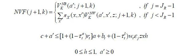
Let denote the value function of a retired worker who is not eligible for pension benefit. The decision problem of this type can be recursively written as

s.t.

The decision rules that solve this problem are , .

Utility Maximization Problem of a Worker

Individual workers begin participating in the labor market at the age of J_W and retire from the market at the age of J_R . Workers are heterogeneous in terms of labor market productivity. Labor market productivity measured in efficiency units is assumed to be composed of three parts. First, a type-dependent fixed effect z is determined at the age of J_W drawn from the probability distribution, π_z(z) . Second, an age-dependent component ε_j is assumed to be deterministic, a persistent idiosyncratic shock x evolves following the conditional probability distribution, π_X(x, x′) . We assume that there is no difference in the labor market productivity structure across generations.3

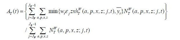
When an individual worker aged j supplies h hours to the labor market, he supplies ε_jzxh units of efficiency labor and earns w_tε_jzxh , where w_t denotes the market wage rate for an efficiency unit of labor in period t . If he is enrolled in the National Pension, his pension contribution is calculated as τ_t min {w_tε_jzxh, y_t} , which is not part of his taxable income under current Korea tax law. Here, τ_t denotes the pension premium rate. The amount of income over the predetermined level y_t is exempt from pension contributions. Hereafter, following the National Pension Act, we refer to y_t as the maximum Standard Yearly Income and min {w_tε_jzxh, y_t} as the Standard Yearly Income. We assume that individual workers begin their economic lives with no financial assets, and borrowing against the future labor income is not allowed.

A worker enrolled in the National Pension is characterized by the state vector (a, p, x, z; j, k) . The variable p denotes his average Standard Yearly Income up to the age of j −1, which summarizes his individual labor income history. Let denote the value function of a worker in the state of (a, p, x, z; j, k) . The decision problem of the agent can be recursively represented as

s.t.

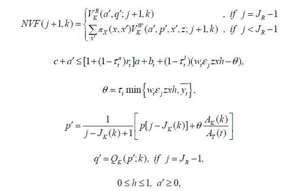
where J_K(k) denotes the age at which k_th cohort workers are enrolled in the National Pension, A_T(t) denotes the Average Yearly Income, which is the average Standard Yearly Income of all insured workers in period t . A_K(k) denotes the three-year average value of the Standard Yearly Income of all k_th cohort workers immediately before their retirement. It is determined using the equation below.

The decision rules that solve this problem are expressed as

The pension contribution reflecting the optimal working hours is denoted as .

As noted above, the amount of the National Pension benefit is determined at the beginning of retirement. Here, we specify how it is determined. The amount of the pension benefits depends on (i) how long a worker contributes to the service, i.e., the insured period, and (ii) how much a worker contributes over the insured period as summarized by his average Standard Yearly Income p . Roughly, the variable p recodes and summarizes the history of labor earnings. Let Q_K(p;k) denote the amount of pension benefits paid to a k_th cohort individual worker with p . Under the modified formula suitable for the model, it is determined as

where n_K(k) denotes the insured period of a k_th cohort worker. The variable D_K(k) determines the income replacement ratio, and it depends on k due to the reforms of the National Pension System in 1998 and 2007.

We now clarify how the average Standard Yearly Income p is determined in the model. The process of calculating the value of p is most easily explained by a simplified example. Suppose there is an insured worker who contributed for T periods before he retires, as shown in Table 1. In period 1, let B₁ be his Standard Yearly Income when the average Standard Yearly Income amounts to A₁ . Let B′₁ denote the reevaluated value of B₁ in the period T , which is determined as B′₁ = B₁×(A_t / A₁). Note that A_T is the Average Standard Yearly Income in period T .4 The multiplying factor A_t / A₁ can be, therefore, interpreted as the cumulative average income growth rate for T periods. If the amount of B₁ is to be put into a saving account for T periods, the bank would roll over B₁ with the market interest rate. What the National Pension does is similar to what the bank does, but it promises to return the savings compounded not with the interest rate but with the labor income growth rate. The future values of B₂, B₃, ⋯ , B_T are determined similarly, which are B′₂, B′₃, ⋯ , B′_T , respectively. Finally, the reevaluated average Standard Yearly Income for the periods during which it is insured is calculated as 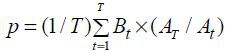, and the period-by-period update formula is shown in the decision problem.

Here, we investigate equation (1) further. The parameter α_A determines the degree of income redistribution within a cohort. If the value of α_A increases, the benefit amount will be closer to the average income among insured people so that the benefit difference among the insured decreases. Conversely, if the value of α_A decreases, the benefit will depend more on the individual earnings history such that the National Pension plays a role similar to that of a bank. The variable D_K(k) in equation (1), known as the income replacement ratio, determines the annual pension payment given the pension contribution history. The value of D_K(k) in equation (1) can be calculated with the officially announced proportional constant d_t . Given the time series of d_t , the value of D_K(k) is calculated as

A worker who is not enrolled in the National Pension is characterized by the individual state vector (a, x, z; j, k)5 Let denote the value function of this type of worker. The decision problem can be recursively represented as

s.t.

The decision rules that solve this problem are denoted as

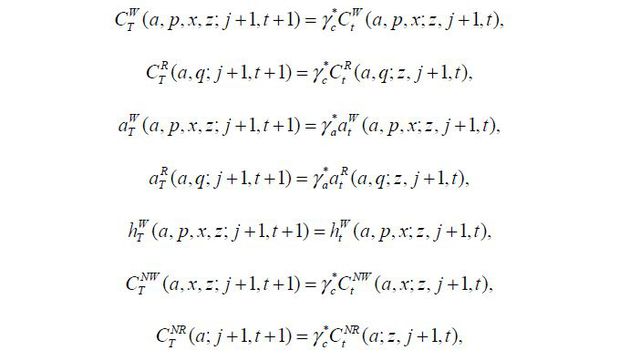
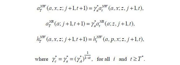
It is convenient to reorder the value functions and the decision rules in the order of time t to construct the macroeconomic variables, as follows:

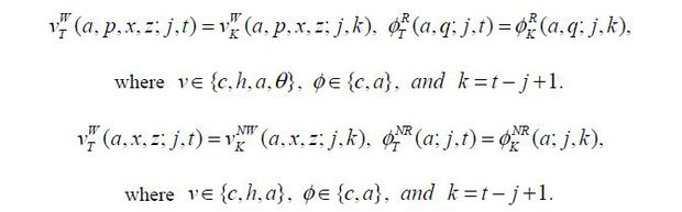
Finally, let (a, p, x, z; j, t) and (a, q; j, t) denote the insured population aged j in period t in the states of (a, p, x, z) and (a, q) , respectively. In the same manner, (a, x, z; j, t) and (a; j, t) denote the population who are not enrolled in the National Pension.

C. The Representative Firm’s Problem

In the model economy, there exists a representative firm which produces output Y_t by combining capital K_t and labor L_t using a constant return-to-scale Cobb-Douglas production function for each time period t ,

where A_t denotes the total factor productivity in period t and α is the output elasticity of capital. The aggregate labor L_t is measured in units of efficiency. Capital stocks are depreciated at the rate of δ_t in period t after production occurs. We assume that both the factor markets and the goods market are competitive.

The firm’s profit maximizing problem can be stated as follows,

where and denote the demand for labor and the demand for capital during period t , respectively. Then, and satisfy the following first-order conditions:

D. Construction of Macroeconomic Variables and Procedure of Market Clearing

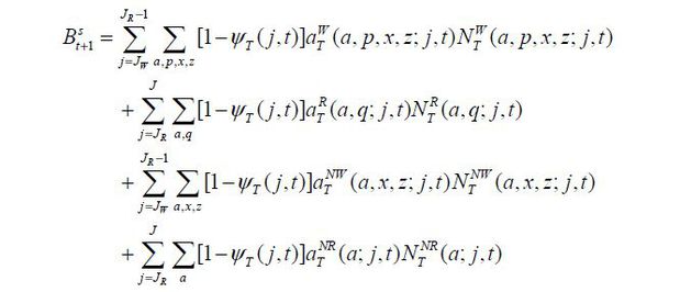
The aggregate supply of capital in period t + 1, is determined by the individuals’ decisions on savings and the evolution of the National Pension Fund. On the one hand, in order to calculate the aggregate savings by individuals, we need to specify how unintended bequests are distributed to living individuals. The amount of assets that the individual aged j in period t in the state of (a, p, x, z) saves is (a, p, x, z; j, t). There are (a, p, x, z; j, t). people in this state. The individual survives in period t +1 with a probability of (1 − ψ_T(j, t)). If a mortality shock arrives, we assume that the assets, (a, p, x, z; j, t), are distributed evenly to the living population. The same process holds for the retired population. Under these assumptions, the aggregate savings by individuals during period t +1 are calculated as follows:

Similarly, the total amount of unintended bequests in period t +1 to living households is calculated as follows:

On the other hand, the National Pension Fund (SF) evolves as follows:

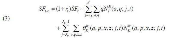
If the National Pension Fund is to be depleted in some period t +1, we assume that the National Pension System switches to a pay-as-you-go system. In this case, the pension premium rate τ_t is endogenously set to ensure the period-by-period budget balance of the National Pension.

We assume that the model economy is closed such that the rate of return on capital is determined in the domestic capital market. Regarding assumption, we rely on the empirical findings of Feldstein and Horioka (1980), who show that the correlation between the investment rate and the savings rate is close to one in the long run. Despite the fact that the open economy assumption is much more realistic for Korea, we would have to project the world interest rate until 2300 to solve the model if such an assumption were to be adopted.6

With the assumption of a closed economy, the aggregate supply of capital in period t + 1, , is the sum of the aggregate savings by individuals and the National Pension Fund.

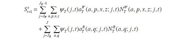
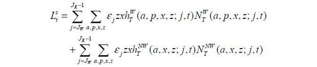
The aggregate supply of labor in period t, , is the sum of efficiency unit of labor supplied by individuals:

The Average Yearly Income in period t, A_T(t), is calculated as follows:

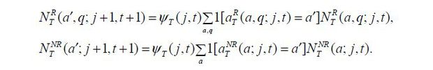
Finally, we need to specify the evolution of the population distribution over the state space. The distribution of the retired population aged j + 1 in period t + 1 is determined as follows: For any asset holdings a′ in period t + 1,

The distribution of the retired population aged J_R in period t + 1 is determined as follows: For any asset holdings a′ and the pension benefits q′ in period t + 1,

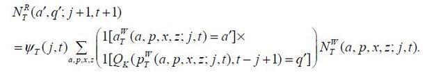
Note that the amount of the pension benefit is being determined for the eligible population aged J_R in period t + 1 .

The distribution of workers aged J_R in period t + 1 who are not eligible for the pension benefit evolves as follows: For any asset holdings a′ in period t + 1,

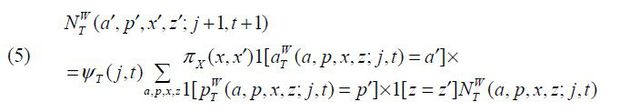
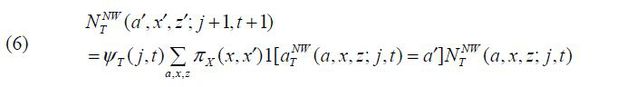
The distribution of the workers aged J_W ≤ J < j_R − 1 in period t evolves as follows: For all combinations of (a', p', x'), (a', x') in period t + 1,

The distribution of the population aged j = J_W in period t + 1 is determined as follows: For any z ,

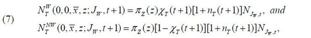
where χ_T(t + 1) denotes the insured rate by the National Pension Service for the birth cohort who will become aged J_W in period t + 1 . Here, x denotes the average value of the persistent part of the individual productivity, x.

E. Definition of the Competitive Equilibrium

Let be the aggregate state of the model economy in period t. We assume that economic agents perfectly foresee the entire path of the state of the aggregate economy, .

Given the path of the aggregate state of the economy, the equilibrium of the economy consists of the value functions ; the associated decision rules , , and the sequence of the production plans for firms {K_t, L_t}; the factor prices {w_t} , {r_t} , the National Pension System {τ_t, y_t, SF_t}; transfer income {B_t}; and the population measures such that

1. Given the path of the aggregate state of the economy and the factor prices, the value functions and the decision rules solve the workers’ dynamic problems.

2. Given the path of the factor prices, {K_t, L_t} denotes the solution to the representative firm’s profit maximization problems.

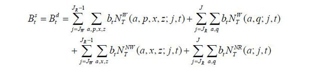
3. Given the path of the factor prices, the factor markets clear and satisfy

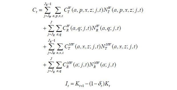
4. The goods market clears as follows: for all t , Y_t = C_t + I_t + G_t, where C_t denotes private consumption, I_t denotes investment, and G_t denotes government expenditures. C_t and I_t are calculated as follows:

5. The National Pension Funds evolves following the equation (3) and switches to a pay-as-you-go system if it is depleted.

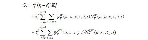
6. The government’s budget maintains a period-by-period balance for all t :

7. The amount of accidental bequests is equal to the amount of transfers to the living population:

8. The distribution of the population over the state space evolves following the equations (4), (5), (6), and (7).

In order to quantify the model economy, we must specify the characteristics of the balanced growth path to which the model economy eventually converges.

First, we assume, in the end, that the net fertility rate and the conditional survival probabilities converge and become constant such that the following conditions are satisfied.

After passing J_D periods upon satisfaction of these conditions, we have

In other words, the growth rate of the total population is equal to the net fertility rate, and the age distribution of the population becomes stationary.

Second, we assume that the growth rate of the total factor productivity converges in the end, i.e.,

Suppose that a stationary population distribution is achieved and that the growth rate of total factor productivity is constant over time. In such a case, the stationary recursive competitive equilibrium is recursive competitive equilibrium in which the following characteristics are satisfied. For all t, the consumption and savings of the representative household increase in proportion and the supply of labor remains constant:

Fourth, the National Pension Service operates as a pay-as-you-go system on the balanced growth path.

Finally, with the conditions above being satisfied, the aggregate supply of savings also increases at a fixed rate and the factor prices are determined as follows:

F. A Welfare Measure

In order to analyze the welfare implications of changes to the National Pension Service, a welfare criterion must be defined beforehand. The welfare function in this study is the total utility obtainable during a lifetime of an individual, which is expected at the time the individual initially become economically active. In order to specify the welfare function, some notations must be introduced.

An allocation of individual consumption and labor supply during a lifetime can be expressed as 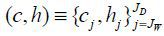.7 The lifetime utility (W) obtainable with this allocation is, then, calculated as 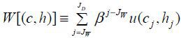. As there is some uncertainty about individual labor productivity, there is also uncertainty in the above allocation. The expected lifetime utility reflecting this uncertainty is expressed as follows and used here as a welfare measure of a given cohort.

This measure has the following characteristics. First, because the consumption of goods and the consumption of leisure are assumed to be normal, the expected lifetime utility increases as the consumption increases or the working hours decreases. Second, the uncertainty of the allocation (c, h) reduces the expected lifetime utility because we assume a risk-averse utility function.

In order to quantify the change in welfare according to a reform of the system, this study applied the certainty equivalent variation, CEV , which can be regarded as the answer to the next question: “In order to avoid a change of the expected lifetime utility after a reform of the system, how much consumption should be increased or decreased from the optimal allocation before the reform?” Specifically, we denote the optimal allocation during a lifetime in the benchmark economy as (c⁰, h⁰) and the optimal allocation in the new equilibrium after a reform as (c^*, h^*) . At this point, the changes in welfare due to institutional changes can be measured as

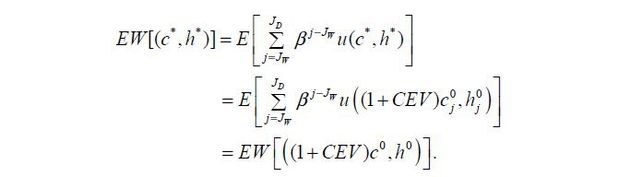
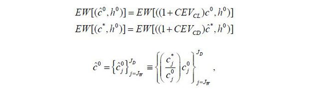
We can decompose CEV into the component (CEV_C) resulting from the change in consumption from c⁰ to c^* and the component (CEV_H) resulting from the change in labor supply from h⁰ to h^* . These components are calculated as follows:8

The part of the welfare change due to the change in consumption schedule, CEV_C , can be further decomposed into a component reflecting the change in the consumption level (CEV_CL) and a component reflecting the change in consumption schedule uncertainty (CEV_CD) as follows:

where and are the average consumption values of the populations whose ages are j before and after the system change, respectively. Similarly, the welfare change due to the change in labor supply, CEV_H , can be divided into CEV_HL and CEV_HD.

A. Demographic Transition

The demographic transition of the model economy is calibrated to match the history and the projection by Statistics Korea as of 2010. To solve the model, projections of fertility and survival probabilities are required to produce the age distribution of the population at each period. The net fertility rates n_T(t) are calculated to match the growth rate of the one-year-old population until 2060. However, to completely solve the model economy quantitatively, we need information beyond 2060. Between 2060 and 2100, the net fertility rate projections are obtained from the Statistical Research Institute. After 2100, they are assumed to be fixed at zero. The conditional survival probabilities, ψ_T(j, t), are drawn from the life tables projected by Statistics Korea. Because the projected life tables are in five-year periods, the probabilities for the interim periods are approximated by linear interpolation. After 2060, the survival probabilities are assumed to remain fixed at the 2060 levels. Under the assumptions specified above, the population distribution reaches a steady state in 2200, wherein the population growth rate is zero percent and the age distribution of the population does not change over time.

B. Utility and Labor Market Productivities

The parameter γ denotes the intertemporal substitution elasticity of work hours. Micro-estimates of γ range from 0.1 to 0.7. We choose a value of 0.4, which is a widely accepted value for the class of the model economy considered in this paper. We choose the weight parameter for disutility from working, B , such that the average number of hours of work is 1/3 between 1989 and 2014 in the model simulation. The preference discount factor β is set such that the average K/Y ratio of the model economy during 1989~2014 matches the average value of the K/Y ratio data for the same period, which is 2.9. Note that the average K/Y ratio of the model economy between 1989 and 2014 is pinned down, but the dynamics is determined endogenously in the model. The definition of the capital stock for calculating the K/Y ratio is the private production capital stock from the National Balance Sheet.

As specified in the previous section, individual workers are heterogeneous along three dimensions that affect their labor productivity: a deterministic age-dependent component , a type-dependent fixed effect z , and a persistent idiosyncratic shock, x . These specifications and the calibration strategy are adopted from Conesa, Kitao, and Krueger (2009). For the type-dependent fixed effect, we consider two ability types z₁ = exp(−σ_z) and z₂ = exp(σ_z) with an equal population mass of 0.5. We assume that E[ln(z)] = 0 and .

For the persistent idiosyncratic shock, we specify the stochastic process such that ln(x) follows the AR(1) process, as follows:

We discretize the AR(1) process with seven nodes using the method suggested by Rouwenhorst (1995). We further assume that x is equal to the unconditional average (≡ x) when workers enter the economy.

The variance of logged productivity is, then, determined along the age dimension as follows:

In order to quantify the specified labor productivity, we need the parameter values for are determined in such way that the model-generated age profile of log earnings in 2014 matches the data. In Figure 3, the age earnings profile from the model simulation is represented by the thick straight line and the calibrated values of put into the model are represented by the thick dashed line. Moreover, the values of , ρ_x, and are calibrated jointly to match the cross-sectional variance of individual labor earnings. As shown in the panel on the right in Figure 3, the cross-sectional variance of logged individual labor earnings increases almost linearly along the age dimension. To mimic this pattern, we must have ρ_x ≈ 1, as implied by equation (8). We, however, limit the value to 0.99 for the parameter ρ_x for technical reasons. The parameter is determined to match the variance for the age of 24, which is 0.1, and the calibrated value is = 0.1. Finally, the parameter is calibrated for the model-generated variance for the age of 60 to match the data, making this value 0.6. The calibrated value for the parameter is 0.016.

C. National Pension System

The National Pension System was introduced in 1988 and has since been revised twice through reforms, in 1997 and in 2007. The model parameters determining the contributions and benefits are calibrated to mimic the current system, which includes the changes put into place by the two reforms. The premium rates are set to 3%, 6% and 9% for the periods of 1988~92, 1993~97, and 1998 onwards, respectively. Note that the system is switching to a pay-as-you-go system if the National Pension Fund becomes insolvent. In such a case, the premium rate is set endogenously to ensure the period-by-period budget constraint. Between 1988 and 1998, the value of α_A was 0.43, but the value has been set to 0.5 since then. The pension reform in 1997, therefore, strengthened slightly the income-redistribution role of the National Pension System.

When the National Pension was introduced, the value of the proportional constant d_t was set to 0.35, which implied an income replacement ratio of 35% for the 20-years-of-enrollment period. As part of the first reform in 1997, the value was lowered to 0.30. With the second reform in 2007, the value of d_t was set to decrease annually by 0.005 until reaching the level of 0.2 in 2028. After 2028, it is assumed to remain fixed at the value of 0.2. Given the time-series of d_t , the values of D_K(k) are calculated using equation (2). Figure 4 reports the calculated income replacement ratios D_K(k) across birth cohorts. When the system was introduced in 1988, an income replacement ratio of 35% after the 20-years-of-enrollment period was targeted, but it is slated to be reduced to the level of 20% eventually. Because the system must honor the previous contributions at the time of the reform, only the future proportional constants had to be decreased to cut the pension benefits, which implied a loss in benefits for the young and for future generations.

In the model economy, the proportion of the insured in each cohort is determined exogenously. For each birth cohort, it is calculated by dividing the number of insured by the number of the population when the cohort reaches the age range of 55~59, as shown in Figure 5. For the 1962~1970 cohort for whom the values are not yet realized, this proportion is assumed to increase to 70%. For those born after 1970, it is assumed to stay at 70%, which is in line with official projections.

The maximum Standard Yearly Income y_t is approximately the twice of the Average Yearly Income A_T(t) in 2014. We assume that this ratio is maintained for all simulation periods.

D. Production function and other parameters

With the Cobb-Douglas production function assumption, if the goods and factor markets are competitive, the output elasticity of capital α turns out to be equal to the capital income share. We choose a value of 0.35, which is the average capital income share between 2000 and 2014. The definition of the capital income share we employ is 1 − (labor income + self-employed income) / GDP .

The total factor productivity (TFP) is calculated with the standard growth accounting method. In this paper, the TFP is assumed to be identified as the Solow residual. Thus, different measures of labor and capital input yield different values of the TFP. To maintain consistency with the model economy, we define the labor input as the total number of employees weighted by the age-productivity profiles. For the future values of total factor productivity, we adopted the TFP growth rate from Cho (2014) until 2035 and assume that there is continued growth thereafter at a constant rate of 1.3 percent per annum. The depreciation rate of capital stock is calculated to match the average private gross real fixed investment of national accounts during the period of 1989 and 2014, which is 29%. The calculated depreciation rate is 8%. We used a value of 5.5% before 2000 to reflect the rising pattern of the depreciation rate in the data. Given the value of the output elasticity of capital of 0.35 and the mean value of the capital-output ratio of 3 after 2000, the implied marginal productivity of capital is about 4% between 2000 and 2015. The labor income tax rate and capital income tax rate are set to 15%.

Model simulations require the initial asset holdings by age in the year 1989. We use Statistics Korea's Household Asset Survey of 2006 to determine the age-asset distribution in 1990; although this survey was conducted for the year 2006, to the best of our knowledge, it is the earliest data available. The aggregate wealth of the model economy in 1989 is then then rescaled to match the K/Y ratio in 1990, which is 2. Within each cohort in the year 1989, the assets are evenly distributed.

A. In-sample Performance of the Model

We compare the simulated aggregate variables with the relevant historical data, in this case the employment growth rate and the real GDP growth rate. Panel A in Figure 6 shows the time series of the GDP growth rate. The model captures the downward trend in the GDP growth well, as the endogenous variables of the model react in a consistent manner with the actual data when the demographic structure and the TFP are fed into the model.

Panel C of Figure 6 depicts the aggregate labor growth rate of the model economy and the employment growth rate from the Economically Active Population Survey.9 Also shown in the figure is the growth rate of the population aged 24~64 in the model economy. The employment growth rate exhibits a slow downward trend and short-run fluctuations. The trend in the employment growth rate is well captured by the growth rate of the population aged 21~64 of the model economy. As reported in Table 2, the contribution of labor to GDP growth was 1.0% per annum in the 1990s and 0.8% per annum in the 2000s. In the model economy, the corresponding numbers are 1.3% and 0.9%, respectively. However, not well replicated by the model economy are the relatively high employment growth rates in the first half of the 2010s. During this period, we observe a slowdown in GDP growth and a relatively high growth rate of employment, resulting in low values of the TFP. In turn, when we feed the realized TFP into the model, it is difficult to generate the high employment growth observed in the data. Part of the problem stems from the fact that we assume that TFP growth accelerates in the second half of the 2010s. Given that agents perfectly foresee the entire path of TFP growth, the working hours chosen by the agents are opposite to what we observe in the data.

Panel D in Figure 6 shows the growth rate of capital stock. Capital stock refers to the share of capital stock held by the private sector from the National Balance Sheet. The long-term downward trend in capital accumulation is also well captured in the model simulation. The secular decline reflects the fact that the slowdown in TFP growth and the decline in the growth rate of the working-age population have lowered the demand for investment. However, the investment boom in the 1990s is not well explained by the model. We view this shortcoming as also stemming partly from the perfect-foresight information assumption. That is, the investment boom during this period may have been based on optimistic expectations for the Korean economy. However, economic agents in the model who perfectly forecast the slowdown in the economy afterwards do not invest as much, as indicated by the data for that period.

Panel B in Figure 6 shows the time series of the capital-output ratio. Because the Cobb-Douglas production function is assumed, the degree to which the capital to output ratio changes is closely related to the changes in the price variables. Shown in Figure 7 are the wage growth rate and the real interest rate. Despite the fact that short-term fluctuations are not well replicated, the trends of these variables are well captured by the model economy, which is crucial for the purpose of this paper. The trend of the model interest rates is similar to that of real corporate bond yields, but these rates have been approximately 1%p higher since the 2000s. The interest rate of the model reflects the marginal productivity of capital, which is not a concept directly comparable to corporate bond yields. However, corporate bond yields are known to be an important variable for forecasting the future fiscal condition of the National Pension, and these are reported here for interested readers.

The growth path of the benchmark model economy, including future projections, is reported in Table 2. To analyze the factors contributing to the secular decline in GDP growth, we also report the results in the growth accounting form. The numbers in parentheses are the growth accounting results based on the data to extract the time series of the TFP. In addition, on the right of the parentheses are the GDP growth projection rates quoted from the Third Long-Term Fiscal Projections in 2013 for comparison.

The ten-year average GDP growth rate of the model economy declines from 6.8% in the 1990s to 4.6% in the 2000s, and to 2.3% in the 2010s, and is projected to stabilize at around 0.7~0.9% after 2050s. The declines in the GDP growth rate are mainly attributable to the decreased contribution of labor input. In the model economy after 2030, the contribution of labor is close to -1%p per annum, which reflects the dramatic decrease in the population aged 21~64. The decline in the working-age population will slow the GDP growth rate further through less accumulation of physical capital. The contribution of physical capital to GDP growth is also steadily declining, reaching only 0.1% per annum in the 2050s. As shown later, the National Pension Fund in the model begins to decline from its peak in 2030 and becomes depleted in 2050. The accumulation of capital is in part negatively affected by the decumulation of the fund from 2030 to 2050.

In the long run, the model economy reaches a balanced growth path, where the population structure and the TFP growth stabilize. As presented in Table 2, total factor productivity increases by 1.3% per annum and physical capital increases by 0.7% per annum. In addition, GDP grows at a rate of 2.0% per annum.

We examine the cross-sectional inequality of income and wealth among economic agents in the model. The panel on the left in Figure 8 shows the Lorenz curve for labor earnings in 2014 from the model. Also shown is the Lorentz curve from actual data (Data) using the Household Finance and Welfare Survey for 2014. The inequality of earned income is slightly lower in the model economy, but the difference is not meaningfully significant. The Gini coefficients of the earned income are 0.35 in the model and 0.38 in the data. The Lorentz curve for wealth is shown in the panel on the right in Figure 8. The degree of wealth inequality is determined endogenously by workers’ optimal choices. It can be seen that the degree of wealth inequality is somewhat greater in the model. In 2014, the Gini coefficient of net asset holdings was 0.58 in the Household Finance and Welfare Survey, but it is 0.64 in the model. The Lorentz curve for wealth indicates that the model generates too many workers with relatively low wealth, which is commonly observed in the class of model applied in this study according to Hugget (1996).

B. Benchmark Model Simulation Results for the National Pension System

In the benchmark model economy, the National Pension Fund reaches its peak in 2030 relative to GDP and runs out of funds in 2049, as reported in Figure 9. After that date, the National Pension System shifts from a partially funded system to a pay-as-you-go system and the equilibrium premium rate soars to a level of 29.3% from the level of 9% in 2050. The premium rate stays at about 30% until 2070 and then falls slightly to 26~27% for a considerable period after 2070. On the balanced growth path, the equilibrium premium rate turns out to be 18.3%, which is still very high compared to the then-current value of 9%. Thus, even without population aging, the 9% premium rate is insufficient to maintain the financial stability of the National Pension System in the benchmark model economy.

In order to examine the generational burden and benefits associated with the current National Pension System in the model, Table 3 reports the average premium rate and the income replacement ratio for selected cohorts. The income replacement ratios are calculated based on 20 years of enrollment. The average premium rate refers to the overall average premium rate during the insured period for each cohort in the model. The drop in the income replacement ratio reflects the two national pension reforms in 1998 and 2007. The average premium rate increases very rapidly for young and future generations because the system switches to a pay-as-you-go system in 2050. The premium rate must skyrocket in order to balance the pension budget in the benchmark model economy. Also reported in Table 3 is the benefits-cost ratio for the selected cohorts. The benefits-cost ratio is defined as the ratio of the present value of the total amount of pension benefits to the present value of the total contributions by a cohort. The present value is calculated with the equilibrium interest rate of the model and is evaluated on the start of economic activity for each cohort. The ratio decreases with the birth cohorts because the income replacement ratio decreases though the premium rate increases. Note that in the long run, the ratio converges not to the level of 1.0 but to the level of 0.8 in the benchmark model simulation.10 Thus, having a profit ratio lower than 0.8, the 2010~2050 cohorts in Table 3 are sacrificing themselves to support the National Pension System in the benchmark model simulation. On the other hand, the earlier birth cohorts benefit from the system.

Choi and Shin (2015) estimated the benefits-cost ratio by cohort based on historical data and the Third Long-Term Fiscal Projections. Their results are shown at the bottom of Table 3 and in Figure 10. In general, our simulation results are consistent with theirs, but the benefits-cost ratio for the 1990 birth cohort is much lower in the benchmark model. This occurs because the premium rate soars when the fund reserve becomes insolvent, whereas Choi and Shin (2015) assume the then-current 9% premium rate to continue indefinitely. In comparison with Choi and Shin (2015), we contend that our model can be considered reasonably successful in replicating the core features of the National Pension System.

A. Increase in the Premium Rate

This subsection reports simulation results to achieve the fiscal stabilization of the National Pension System by raising the premium rate. Because there is no explicit agreement on the definition of fiscal stabilization as it pertains to the National Pension System, we adopt the definition suggested by the Third National Pension Improvement Committee in 2013. It suggested as a goal to maintain a reserve fund at more than twice the projected annual expenditure until 2083. In this subsection, we calculate the equilibrium premium rate necessary to remain solvent for another 30 and 50 years from the date of the depletion in the benchmark model economy. More specifically, we find the minimum premium rates that allow the National Pension Fund to avoid depletion until 2080 (Plan 1) and 2100 (Plan 2). We then analyze the welfare consequences based on the welfare criterion presented in Section 3. To simplify the problem, we assume that the government will announce a one-time unexpected premium rate increase in 2021 and implement the plan immediately. Reported in the left panel of Figure 11 is the equilibrium premium rate after the reforms. It was found that is necessary to raise the premium rate by 9.3%p for Plan 1 and 11.0% p for the Plan 2 from the current premium rate of 9%.

The macroeconomic effects of the Plan 1 are reported in Table 4. The numbers reported in Table 4 are the percentage deviation in levels from the benchmark model for the selected years. The numbers in the parentheses are the simulation results, in which the wage growth rate and the interest rate are fixed at the level of the benchmark model.

If the price variables are not allowed to vary, the capital stock increases by 19.2% in 2060 compared to the benchmark model mainly due to the large increase in the National Pension Fund. In the long run, the capital stock, however, converges to the level of the benchmark model given that Plan 1 is only a temporary measure.

The labor supply is low relative to the benchmark model until 2049, when the fund depletes in the benchmark model. However, the labor supply increases significantly between 2050 and 2080 in response to the drop in the premium rate compared to the benchmark model. Like the capital stock, the labor supply returned to the same level as the benchmark economy in the long run. With regard to GDP, the effect of the increase in the capital stock outweighs that of the decrease in the aggregate labor input. Therefore, output also increases except for a few periods immediately after the implementation of Plan 1.

In the general equilibrium case, the adjustments in prices to clear markets significantly dampen the response of the macroeconomic variables. As the National Pension Fund expands, the equilibrium interest rate falls sharply as capital stock relative to labor input increases rapidly. The equilibrium interest rate falls by 0.5%p in 2060, when its difference reaches the maximum. On the other hand, the increased wages induce workers to supply more labor to the market. The expansionary output effect reaches its maximum relative to the benchmark simulation in 2050, and the GDP increases by 4.3%. To increase the GDP by 4.3% in 30 years, it must grow more rapidly by approximately 0.15% per annum from 2021 to 2050, which is a significant growth effect given the low growth rate projection in the benchmark model economy. The macroeconomic effects of the implementation of Plan 2 are reported in the appendix. In order to facilitate comparison with Plan 1, the results for Plan 1 are reported again in the parentheses.

Table 5 shows the changes in the average premium rate and the benefits-cost ratio according to Plan 1 and Plan 2. Recall that the equilibrium premium rate to implement Plan 1 is 18.2%. Because the transition to the pay-as-you-go system is delayed for 30 years, the equilibrium premium rates between 2050 and 2080 drop significantly. As a result, the average premium rates during a lifetime for the generations working for that period are significantly lower. For example, the average premium rate for the 2030 cohort fell by 7.1%. However, the effect on the average premium rate for the 2050 cohort was insignificant, as they start working in the mid2070s. As shown in Figure 11, Plan 1 is not a long-term solution to the fiscal problems of the system, though it postpones the depletion of the fund. On the other hand, the average premium rate for the generations born before 2000 increases due to the reform. For example, in case of the 1980 cohort, the average premium rate rises by 5.3%p by Plan 1, which is still lower than the long-run steady state premium rate of 18.3%.

With the implementation of Plan 2, the fund’s insolvency is postponed until 2100 and the premium rate rises to 20%. As shown in the panel on the right in Figure 11, the premium rate and the benefits-cost ratio are greatly equalized across generations, despite the fact that Plan 2 does not avoid the depletion of the reserve fund. Note also that the benefits-cost ratios for the young and future generations become similar to the long-run steady-state value under Plan 2.

We now turn to look at the welfare implications of the reforms. The change in welfare in terms of CEV for the selected birth cohorts are reported in Table 6 and Table 7. The patterns of welfare changes among the generations are similar to the changes in the average premium rate reported in Table 5. The welfare of the 2020~2050 cohorts, who supply labor actively between 2050 and 2080, increases significantly due to the reform as the burden of paying a premium falls sharply. For example, the welfare gain of the 2030 cohort is found to be 9.3% in terms of CEV , which means that the gain amounts to an increase in consumption of 9.3% for every possible contingency during the lifetime of this cohort. Note that most of the welfare change is explained by the increase in consumption, CEV_C . Further decomposition of CEV_C shows that the gain from the reduction in uncertainty, CEV_CD is negligible relative to CEV_CL . However, note that CEV_CD is positive for the 2030~2050 cohorts; moreover, the magnitude is not too small so as to be ignored. As the average premium rates for these cohorts drop sharply, their ability to accumulate savings to buffer the effects of productivity shocks on consumption is improved significantly.

The decomposition of welfare change shows that for the young and future generations, the reduction in the burden to support the National Pension System greatly improves their welfare. Of course, they benefit from the reform at the expense of the older generations. However, the welfare analysis in Table 6 together with the changes in the benefits-cost ratios reported in Figure 11 clearly indicate that the current system is unjustifiably partial to those in the older generations.

Shown in Table 7 are the welfare changes caused by the implementation of Plan 2. As expected, the results are qualitatively similar to those of Plan 1 and are quantitatively larger than those of Plan 1. However, the results in Table 5 are interpreted as meaning that Plan 2 distributes more evenly the burden of supporting the National Pension System than Plan 1 across generations, as the benefits-cost ratios become closer to the steady-state value for many more generations. However, in the model economy, older cohorts that start working before 2021 lose due to the reforms. If the implementations of Plans 1 and 2 are determined by voting in 2021, it turns out that even Plan 1 is not implementable, as the future generations are not eligible to vote.

We also attempted to find ways to achieve the goal of Plan 1 by reducing the benefits of the National Pension, i.e., by adjusting the proportional constant d_t . However, if the system is to be modified akin to how the second National Pension reform was in 2007, this goal cannot be achieved. The reform in 2017 guaranteed proportional constants before the reform and announced a lowering of the proportional constants for the years to come. By honoring this vested right, we could not achieve the goal of postponing the depletion of the reserve fund for 30 years.

B. Strengthening Income Redistribution

As noted in the previous section, the degree of income redistribution is determined by the weight parameter α_A in equation (1). If the weight parameter were 1, regardless of individual earnings histories, the amounts of pension benefits would be identical for all beneficiaries within a birth cohort. At the other extreme, if the weight parameter were 0, the amount of pension benefits only depends on the individual earnings history, and there would not be any income redistribution by the National Pension System. In this subsection, the change in welfare is measured when the weight parameter changes to the value of 0.99 from the current value of 0.5. As the value of α_A increases, it turns out that the welfare evaluated by CEV for future generations increases. Therefore, we only report the simulation results of α_A being equal to the value of 0.99. We assume that the government will announce unexpectedly the change in the weight parameter in 2021 and implement it immediately in that year. We further assume that only the beneficiaries who retire after the announcement are affected by the reform. We refer this reform as Plan 3 hereafter.

The macroeconomic effects of Plan 3 are summarized in Table 8. As in Table 4, the percentage deviations in levels from the benchmark simulation are reported. Unlike the fiscal stabilization plans in the previous subsection, the reform in this subsection changes the system permanently and the macroeconomic variables are affected even in the long run. The aggregate labor supply and savings increase, resulting in an increase in the total output compared to the benchmark model. The wage rate is higher and the interest rate is lower than in the benchmark simulation as the aggregate labor supply relative to capital stock increases.

Researchers who are familiar with the class of model in this paper may see the results shown in Table 8 as counterintuitive. Because the uncertainty about allocation is expected to decrease due to the reform, the workers directly affected by the reform would supply less and save less as the precautionary motive decreases. However, the results in Table 8 are considered to be a somewhat special case because there is an upper limit on the Standard Yearly income (y_t) . We checked the case in which there is no maximum Standard Yearly Income in equation (1). In that model economy, the reform caused decreases in the labor supply, savings and output.

Reported in Table 9 are the changes in welfare in terms of CEV for the selected cohorts who start working after 2021. The welfare increases for all cohorts in Table 9 and the improvement show consumption increases of approximately 1.5% to 2.2% for every possible contingency compared to the benchmark economy. This increase in expected lifetime utility is attributable to the increase in consumption (CEV_C) rather than to a change in working hours. However, unlike the effects of fiscal stabilization reforms, the improvement in welfare arises from a reduction in the uncertainty of consumption path (CEV_CD) as opposed to being an effect of the level of consumption (CEV_CL).This result implies that in addition to the self-insurance mechanism through adjustments to the labor supply and savings, the National Pension System plays a role in providing additional insurance from labor market productivity shocks. Given the calibrated labor income process, workers in the benchmark economy desire more insurance to be provided by the National Pension System, which is reflected in the increase in the expected lifetime utility by the reform. The majority (64.3%) of the current population in 2021 are found to be in favor of the reform in the benchmark model simulation.

References

, , & (2007). Global Demographic Trends and Social Security Reform. Journal of Monetary Economics, 54(1), 144-198, https://doi.org/10.1016/j.jmoneco.2006.12.010.
, , & . (2009). Taxing Capital? Not a Bad Idea After All. American Economic Review, 99(1), 25-48, https://doi.org/10.1257/aer.99.1.25.
, , & (2010). The Macroeconomic Implications of Rising Wage Inequality in the United States. Journal of Political Economy, 118(4), 681-722, https://doi.org/10.1086/656632.
. (1996). Wealth Distribution in life-cycle Economies. Journal of Monetary Economics, 38, 469-494, https://doi.org/10.1016/S0304-3932(96)01291-3.
, & . (2008). Effects of Fiscal Policy on Labor Markets: A Dynamic General Equilibrium Analysis. KDI Journal of Economic Policy, 30(2), 185-224, in Korean, https://doi.org/10.23895/kdijep.2008.30.2.185.
, & . (2007). On the Consequences of Demographic Change for Rates of Returns to Capital, and the Distribution of Wealth and Welfare. Journal of Monetary Economics, 54, 49-87, https://doi.org/10.1016/j.jmoneco.2006.12.016.
. (2017). Korea’s Demographic Transition and Long-Term Growth Projection Based on an Overlapping-generations model. KDI Journal of Economic Policy, 39(2), 25-52, https://doi.org/10.23895/kdijep.2017.39.2.25.
, & . (2007). Does Social Security Privatization Produce Efficiency Gains? Quarterly Journal of Economics, 122(4), 1677-1719, https://doi.org/10.1162/qjec.2007.122.4.1677.