- P-ISSN 2586-2995
- E-ISSN 2586-4130

We estimate three continuous-time stochastic volatility models following the approach by Aït-Sahalia and Kimmel (2007) to compare the Korean and US stock markets. To do this, the Heston, GARCH, and CEV models are applied to the KOSPI 200 and S&P 500 Index. For the latent volatility variable, we generate and use the integrated volatility proxy using the implied volatility of short-dated at-the-money option prices. We conduct MLE in order to estimate the parameters of the stochastic volatility models. To do this we need the transition probability density function (TPDF), but the true TPDF is not available for any of the models in this paper. Therefore, the TPDFs are approximated using the irreducible method introduced in Aït-Sahalia (2008). Among three stochastic volatility models, the Heston model and the CEV model are found to be best for the Korean and US stock markets, respectively. There exist relatively strong leverage effects in both countries. Despite the fact that the long-run mean level of the integrated volatility proxy (IV) was not statistically significant in either market, the speeds of the mean reversion parameters are statistically significant and meaningful in both markets. The IV is found to return to its long-run mean value more rapidly in Korea than in the US. All parameters related to the volatility function of the IV are statistically significant. Although the volatility of the IV is more elastic in the US stock market, the volatility itself is greater in Korea than in the US over the range of the observed IV.
Continuous-time Stochastic Volatility Model, Integrated Volatility Proxy, Maximum Likelihood Estimation
C22, C51, C58
Researchers such as Lee and Yu (2018), Choi and Cho (2017), and Yoon (2007) have reported evidence that Korean and US share prices move together using a variety of discrete- time econometric models. In addition, Kim (2010), Lee and Ryu (2013), Han et al. (2015), and Cho et al. (2015) studied the statistical properties of the VKOSPI and/or the VIX and suggested models to predict these. On the other hand, continuous-time diffusion models are widely employed to model and investigate the dynamics of stock prices. Diffusion models have been useful for stock prices because using them makes it more convenient to evaluate derivatives. Therefore, it is important and interesting to find a diffusion model that can describe the evolutions of stock prices well and to determine if two markets behave similarly in the context of a continuous-time model. The aim of this paper is not to look into the existence of co-movement in Korean and US stock prices but to estimate several stochastic volatility models for each country to find which one fits the data better. Moreover, we compare these two stock markets based on the estimation results to check whether or not the two countries' stock prices move analogously.
Although the Black-Scholes-Merton model (Black and Scholes, 1973; Merton, 1973) has been adopted quite often in descriptions of the dynamics of stock prices since the 1970s, researchers have found that this model is incapable of explaining certain stylized features of stock prices. These include the time-varying instantaneous volatility of stock prices and the phenomenon by which stock prices become more volatile when they decrease, well known as the leverage effect. Moreover, the implied volatility of options varies with time to maturity, strike prices, and maturities (Stein, 1989; Aït-Sahalia and Lo, 1998), which cannot be true if the stock price follows geometric Brownian motion. To address these issues, researchers have proposed a variety of continuous-time stochastic volatility models. Examples can be found in Hull and White (1987), Stein and Stein (1991), Heston (1993), and Lewis (2000).
Aït-Sahalia and Kimmel (2007) demonstrated that estimating continuous-time stochastic volatility models by maximum likelihood estimation (MLE) with approximate log-likelihood expansions produces accurate estimates of the parameters. In doing so, they generate and use an integrated volatility proxy for the latent volatility variable with the implied volatility of short-dated at-the-money option prices. Following their approach, we apply their estimation procedure to three stochastic volatility models, the Heston, GARCH and CEV (constant elasticity of volatility) processes, to compare the Korean and US stock markets. For the stock price and the implied variance of an at-the-money option with a maturity of 30 calendar days, the Korea Composite Stock Price Index 200 (KOSPI 200) and the VKOSPI for Korea and Standard & Poor's Composite 500 stock index (S&P 500 Index) and the VIX for the US were utilized. The data period is from April 13, 2009 until July 28, 2017, as the VKOSPI data series started to be announced on April 13, 2009, whereas more data are available for the other variables.
We conduct MLE in order to estimate the parameters of the stochastic volatility models considered in this paper. To do this we need the transition probability density function (TPDF). However, as is often the case even for a univariate diffusion process, the true TPDF is not available for any of the models in this paper. Although the true TPDFs of the stochastic volatility processes are unavailable, we can approximate them fairly accurately owing to Aït-Sahalia (2008), who suggests a method to approximate the true TPDF of a multivariate time-homogeneous diffusion model. Using the fact that the TPDF satisfies Kolmogorov forward and backward partial differential equations (PDEs), Aït-Sahalia (2002) and Aït-Sahalia (2008) respectively developed new ways to obtain an approximate TPDF of a univariate diffusion model and a log-TPDF expansion of a multivariate diffusion model in a closed form in the time-homogeneous case. His idea was extended to univariate time-inhomogeneous diffusion models by Egorov, Li, and Xu (2003); to multivariate time-inhomogeneous diffusion models by Choi (2013) and Choi (2015b); to a damped diffusion model by Li (2010); to a multivariate time-homogeneous jump diffusion model by Yu (2007), and to a multivariate time-inhomogeneous jump diffusion model by Choi (2015a). Other related papers include those by Bakshi, Ju, and Ou-Yang (2006); Stramer, Bognar, and Schneider (2010); and Chang and Chen (2011).
Among the three stochastic volatility models investigated, the Heston model and the CEV model are found to be best for the Korean and US stock markets, respectively. Based on these estimation results, we find that there exist relatively strong leverage effects in both countries. Even if the long-run mean level of the integrated volatility proxy (IV) was not statistically significant in either market, the speeds of the mean reversion parameters are statistically significant and meaningful in both. The IV is found to return to its long-run mean value more rapidly in Korea than in the US. All parameters related to the volatility function of the IV are statistically significant. The elasticity of the volatility of the IV is 0.50 for Korea and 0.62 in the US. Although it is more elastic in the US stock market, the volatility itself is greater in Korea than in the US over the range of the observed IV.
Looking at the overall estimations results, most parameters of the stochastic volatility models are quite accurately estimated for both countries. Furthermore, stochastic volatility models can capture well-known characteristics of share prices in both countries. This implies that introducing another stochastic factor for the instantaneous volatility of stock prices is desirable for a better fit of the data for both Korea and the US. Therefore, the stochastic volatility model appears to be more appropriate than the Black-Scholes-Merton model in explaining the movements of stock prices at least for these two countries.
The rest of this paper is organized as follows. We discuss certain features of the data and how to obtain a volatility proxy from the implied volatility. The next section introduces the three continuous-time stochastic volatility models employed in this article. After explaining the estimation method and how to derive the approximate log-likelihood for our models in Section IV, the estimation results and discussions are presented in Section V, after which we conclude the paper.
Daily time-series data of the Korea Composite Stock Price Index 200 (KOSPI 200) and the VKOSPI for the Korean stock market and those of Standard & Poor's Composite 500 stock index (S&P 500 Index) and the VIX for the US stock market were attained from Datastream for the period from April 13, 2009 to July 28, 2017. To compare the Korean and US stock markets, we used the same data period. Although the S&P 500, VIX, and KOSPI 200 data are available before April 13, 2009, we chose this data period because data for the VKOSPI series started to be released only on April 13, 2009.
The S&P 500 Index is a market-value weighted index of 500 large firms in the US and it is known to represent the U.S. stock market well. The Chicago Board Options Exchange (CBOE) publishes the VIX, which is an index of the implied volatility of options on the S&P 500. The VIX is calculated using a variety of 30-day European call and put options on the S&P 500 traded in the market. The KOSPI 200 is computed as the current market value of 200 large companies in Korea divided by the base market capitalization as of January 3, 1990. Because the KOSPI 200 accounts for more than 70% of the market value of all stocks in the KOSPI, it is a good measure of movements in the Korean stock market. Since April 13, 2009, the Korea Exchange (KRX) has calculated the VKOSPI using a method very similar to that of the VIX and has reported it to the public. The VKOSPI is the implied volatility of European call and put options on the KOSPI 200. See Choi and Han (2009) for more about the VKOSPI. As shown below, we take the logarithm of the stock price and construct a proxy for the volatility process of the stock price with the implied volatility to estimate the stochastic volatility models. The true instantaneous volatility variable is unobservable, and we use a proxy in place of this variable. Aït-Sahalia and Kimmel (2007) propose a means by which to create a volatility proxy out of the implied volatility utilizing an idea by Hull and White (1987) (see also Jones (2003)). This is referred to as the integrated volatility proxy (IV). Under a risk-neutral measure, the drift of the volatility process Vt for all models estimated here takes the form a + bVt , where a and b are constants. In this case, we are able to obtain the integrated volatility proxy IVt according to
where  is the observed implied variance of an at-the-money option with a short-maturity
τ. In our case is (VKOSPIt / 100)2 and (VIXt / 100)2 for the Korean and US stock markets, respectively.
is the observed implied variance of an at-the-money option with a short-maturity
τ. In our case is (VKOSPIt / 100)2 and (VIXt / 100)2 for the Korean and US stock markets, respectively.
In estimating the stochastic volatility models, we utilize a two-stage estimation procedure. The first stage estimation involves estimating the univariate CEV model for each case of (VKOSPIt / 100)2 and (VIXt / 100)2. For Korea (the US), we estimate
with Yt = (VKOSPIt / 100)2 (Yt = (VIXt / 100)2) to acquire a = κγ and b = −κ in equation (1). Using these and  or (VKOSPIt / 100)2 and setting τ = 22 / 252 because the time to maturity is 22 trading days (or 30 calendar days),
we can construct the integrated volatility proxy, IVt through equation (1) for both countries.1 The method of maximum likelihood estimation is adopted to determine the parameter
estimates of (2). In doing so, it is necessary to have the transition probability
density function (TPDF) of model (2) but the true TPDF is unavailable. Therefore,
we make use of the irreducible method in Aït-Sahalia (2008) to obtain an approximate transition log-likelihood function of diffusion process
(2).2
or (VKOSPIt / 100)2 and setting τ = 22 / 252 because the time to maturity is 22 trading days (or 30 calendar days),
we can construct the integrated volatility proxy, IVt through equation (1) for both countries.1 The method of maximum likelihood estimation is adopted to determine the parameter
estimates of (2). In doing so, it is necessary to have the transition probability
density function (TPDF) of model (2) but the true TPDF is unavailable. Therefore,
we make use of the irreducible method in Aït-Sahalia (2008) to obtain an approximate transition log-likelihood function of diffusion process
(2).2
Maximum likelihood estimates of the parameters of (2) and the formula used to determine IVt for Korea and the US are provided in Table 1. For both countries, all parameter estimates are statistically quite significant. Comparing the Korean and US implied volatilities based on the estimation results, both the speed (κ) and the long-run average level (γ) to which the implied volatility reverts are greater in the US than in Korea. The parameter estimates of σ and β reveal that the VIX is more volatile than the VKOSPI and that the elasticity of the volatility of the implied volatility with respect to the implied volatility is close to 1 for both countries. The integrated volatility proxy formula is calculated through equation (1) and provided directly below each country's estimation results.
Note: Maximum likelihood estimates of the parameters of the univariate CEV model for the VKOSPI and the VIX and their standard errors in parentheses are given in this table. The two asterisks next to the estimate indicate statistical significance at the 1% level. Directly below each country's estimation results, the integrated volatility proxy formula is calculated through equation (1) and provided.
Figure 1 displays daily time-series plots of KOSPI 200 and VKOSPI from April 13, 2009 to July 28, 2017. The left y-axis is for the KOSPI 200 plot in blue and the right y-axis is for the VKOSPI plot in red. A visual inspection of Figure 1 indicates that the implied volatility tends to increase, particularly when the stock price falls. This phenomenon is well known as the leverage effect. The sample correlation between the KOSPI 200 and VKOSPI in Table 2 is −0.60, which confirms the leverage effect in the Korean stock market. We also note that the VKOSPI tends to revert to a certain level, which we refer to as the long-run mean.
Note: Daily observations of the KOSPI 200 and the VKOSPI data from April 13, 2009 to July 28, 2017 are depicted in Figure 1. The left y-axis is for the KOSPI 200 plot in blue and the right y-axis is for the VKOSPI plot in red.
Note: Descriptive statistics for the daily KOSPI 200, the VKOSPI, ln(KOSPI 200) , and the integrated volatility from April 13, 2009 to July 28, 2017 are computed. Here, the skewness coefficient μ3 / σ3 and the excess kurtosis μ4 / σ4 − 3 are respectively normalized measures of the asymmetry and the thickness of the tails of the distribution relative to the standard normal distribution. Note that for a random variable Xt, μi = E [(Xt - μi)] and σ2 = E [(Xt - μ)2].
In the top panel of Figure 2, daily changes in the KOSPI 200 and the VKOSPI data are plotted. Here, the left y-axis and the right y-axis denote the changes in the KOSPI 200 and the VKOSPI, respectively. This figure shows that the implied volatility increases with the variance in the stock price. Daily changes in the VKOSPI graphed in the bottom panel of Figure 2 verify that the variability of the implied volatility is likely to increase as the implied volatility increases. Stochastic volatility models are capable of capturing these characteristics.
Note: In the top panel of Figure 2, daily changes in the KOSPI 200 and the VKOSPI data are plotted. Here, the left y-axis and the right y-axis denote the changes in the KOSPI 200 and the VKOSPI, respectively. Daily changes in the VKOSPI are graphed in the bottom panel of Figure 2.
Descriptive statistics pertaining to the daily KOSPI 200 and the VKOSPI, ln(VKOSPI) , and the integrated volatility from April 13, 2009 to July 28, 2017 are computed in Table 2. Here, the skewness coefficient, μ3 / σ3 and the degree of excess, μ4 / σ4 − 3 are respectively normalized measures of the asymmetry and the thickness of the tails of the distribution relative to the standard normal distribution. Note that for a random variable Xt, μi = E [(Xt - μi)] and σ2 = E [(Xt - μ)2]. Both the skewness coefficient and the degree of excess imply that none of these data series have normal distributions. Negative strong correlations between the KOSPI 200 and the VKOSPI, and ln(VKOSPI) and the IV, show there is a strong leverage effect in the Korean stock market. Again, what we use to estimate the stochastic volatility models are ln(VKOSPI) and the IV. Integrated volatility is nothing but a linear transformation of implied volatility, which does not affect the correlation, whereas taking the logarithm of the KOSPI 200 does. Even so, there is a solid negative correlation between ln(VKOSPI) and the IV.
Similarly to Figure 1, Figure 3 depicts the daily observations of the S&P 500 and the VIX from April 13, 2009 to July 28, 2017. The left y-axis is for the S&P 500 plot in blue and the right y-axis is for the VIX plot in red. We can observe a greater leverage effect in the US stock market than in the Korean stock market. Looking at Table 3, the sample correlation between the S&P 500 and the VIX is negative and greater than the corresponding Korean correlation in terms of the absolute value. The same is true for ln(S & P 500) and the IV.
Note: Daily observations of the S&P 500 and the VIX from April 13, 2009 to July 28, 2017 are depicted in Figure 3. The left y-axis is for the S&P 500 plot in blue and the right y-axis is for the VIX plot in red.
Note: Descriptive statistics for the daily S&P 500, the VIX, ln(S & P 500) and the integrated volatility from April 13, 2009 to July 28, 2017 are computed. Here, the skewness coefficient μ3 / σ3 and the excess kurtosis μ4 / σ4 − 3 are respectively normalized measures of the asymmetry and the thickness of the tails of the distribution relative to the standard normal distribution. Note that for a random variable Xt, μi = E [(Xt - μi)] and σ2 = E [(Xt - μ)2].
The top panel in Figure 4 depicts the daily changes in the S&P 500 and the VIX data. Here, the left y-axis is for the changes in the S&P 500 and the right y-axis is for the VIX. Daily changes in the VIX are graphed in the bottom panel of Figure 4. As in Figure 2, the changes in both the S&P 500 and the VIX are considerable, especially when the level of the VIX is high. This demonstrates that the volatility of stock prices depends on the implied volatility and that the volatility of the implied volatility appears to be an increasing function of the implied volatility.
Note: In the top panel of Figure 4, daily changes in the S&P 500 and the VIX data are plotted. Here, the left y-axis and right y-axis are for the changes in the S&P 500 and the VIX, respectively. Daily changes in the VIX are graphed in the bottom panel of Figure 4.
We tabulate summary statistics of the S&P 500, the VIX, ln(S & P 500)and the IV in Table 3. Examining the skewness coefficient and the degree of excess of all US data, they are far from normal. There exist leverage effects in the US stock market, and they are stronger than those in the Korean market because the sample correlations between the S&P 500 and the VIX and ln(S & P 500) and IV are all negative and closer to −1 than those for Korea.
Although we have discussed certain features of the Korean and US stock market data using data plots and descriptive statistics, it is more important to check if we can find any evidence to support the observations by estimating with appropriate econometric models, such as stochastic volatility models.
Three different continuous time stochastic volatility models have been used to describe the dynamics of the data. These are the Heston, GARCH and CEV models. The former two are nested by the CEV model.
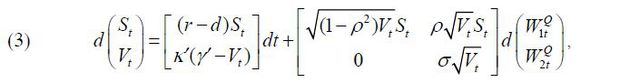
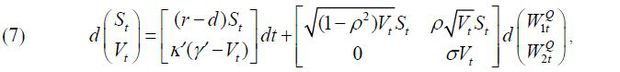
The Black-Scholes-Merton model (Black and Scholes, 1973; Merton, 1973) has been quite popular because it provides a closed-form formula for a European option on an asset. In this model, the underlying asset price follows geometric Brownian motion which is, however, known not to explain the movements of this type of data well. To improve upon the Black-Scholes-Merton model Heston (1993) suggests the following stochastic volatility model.
where  and
and  are independent Brownian motions under the risk neutral measure. And r is the instantaneous risk-free interest rate and d is the instantaneous dividend yield of the stock. As noted in the previous section,
there is some evidence that continuously compounded stock returns are not normal and
that their variances are not constant for the KOSPI 200 and the S&P 500 data. For
this reason, the variance process Vt is introduced for the variance of St. In addition, the stock price is allowed to be correlated with the variance. The
parameter ρ measures the correlation between St and Vt. The volatility process Vt obeys the square root process of Feller (1952), and Feller’s condition 2k'γ' ≥ σ2 must hold for the variance Vt to be positive.
are independent Brownian motions under the risk neutral measure. And r is the instantaneous risk-free interest rate and d is the instantaneous dividend yield of the stock. As noted in the previous section,
there is some evidence that continuously compounded stock returns are not normal and
that their variances are not constant for the KOSPI 200 and the S&P 500 data. For
this reason, the variance process Vt is introduced for the variance of St. In addition, the stock price is allowed to be correlated with the variance. The
parameter ρ measures the correlation between St and Vt. The volatility process Vt obeys the square root process of Feller (1952), and Feller’s condition 2k'γ' ≥ σ2 must hold for the variance Vt to be positive.
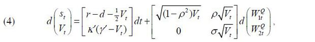
Expressing (3) in terms of st = In St and Vt, we obtain
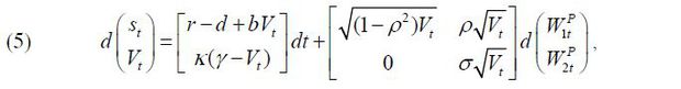
due to Ito’s lemma. As in Aït-Sahalia and Kimmel (2007), we specify the market prices of risks as  . Then, according to the Girsanov theorem, the joint dynamics of st and Vt under the objective measure P are determined by
where  , κ = κ' − λ2σ, and
  . One problem with (5) is that we cannot identify both λ1 and λ2 when we estimate the parameters of model (5) using the maximum likelihood estimation
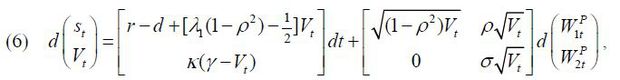
(MLE) method. To resolve this issue, we set λ2 = 0 following Aït-Sahalia and Kimmel (2007). Model (5) reduced to
. One problem with (5) is that we cannot identify both λ1 and λ2 when we estimate the parameters of model (5) using the maximum likelihood estimation
(MLE) method. To resolve this issue, we set λ2 = 0 following Aït-Sahalia and Kimmel (2007). Model (5) reduced to
Thus, the parameter vector we need to estimate is θ = (κ, γ, σ, ρ, r, λ1). The parameter κ indicates the speed of the mean reversion of Vt to its long-run mean level, γ and the parameter ρ measures the correlation between the innovations of the stock price and the volatility. We hold that there is a leverage effect when it takes a negative value.
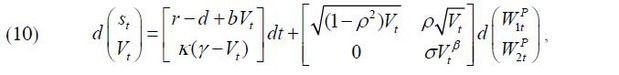
Another interesting model examined here is the GARCH model (Nelson, 1990; Meddahi, 2001). In this case, the stock price and its variance follow
under the risk-neutral measure. The lone difference between the Heston model and the
GARCH model is that the volatility function of Vt for the latter is Vt while it is  for the former. The condition κ'γ' ≥ 0 is required to ensure positivity of the variance Vt.
If we write model (7) in terms of (st, Vt) we obtain the following with Ito’s lemma:
Using the same market price specification,  as above, (st, Vt) obeys
under the physical measure P, where  , κ = κ', and γ = γ'. The resulting model (8) contains the same set of parameters appearing in model (6).
This model is also nested by the CEV model below.
, κ = κ', and γ = γ'. The resulting model (8) contains the same set of parameters appearing in model (6).
This model is also nested by the CEV model below.
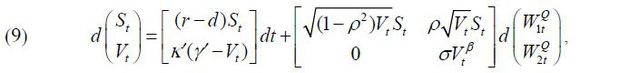
The final model we consider is the CEV model.
The two models above are encompassed by this model given that we have the Heston model when β = 1/2 and the GARCH model when β = 1. Chan, Karolyi, Longstaff, and Sanders (1992) proposed the constant elasticity of volatility (CEV) model for short-term interest rates. In this model, the volatility of the volatility process Vt follows the CEV process, which is why we refer to this model as the CEV model. Note that the parameter β indicates the elasticity of the volatility of Vt with respect to Vt. Lewis (2000) and Chacko and Viceira (2003) also adopted the CEV model for the volatility variable.
Again, if we write model (9) in terms of (st = ln(St, Vt),
With the same assumption for the market prices of risk, as in the Heston and GARCH models, according to the Girsanov theorem, the dynamics
of the state variables are expressed as
where , κ = κ', and γ = γ'. under the physical measure P. We impose the restriction 1/2 ≤ β ≤ 1to ensure the uniqueness of option prices, as in Aït-Sahalia and Kimmel (2007).
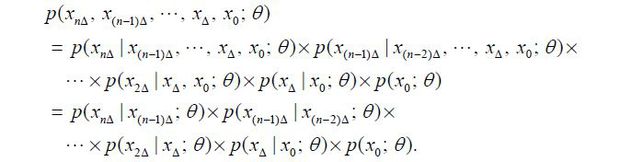
To estimate the models considered in this paper, we use the maximum likelihood estimation (MEL) method. We only have discrete data for the continuous-time process, Xt = (st, Vt) at discrete time points t = iΔ where i = 0, 1, 2,···, n. The joint probability density function (pdf) of the data (xnΔ, x(n−1)Δ, xΔ, x0) is then
Here the first equality is due to the Bayes' rule and the second equality stems from the Markov property of a diffusion process. Taking the logarithm of the joint pdf and ignoring the initial observation, the log-likelihood function is written as
Therefore, in order to carry out MLE, it is critical to have the transition density or log- likelihood function of stochastic volatility models. Unfortunately, the true transition density function is not known for any of the models we use in this paper, as is often the case for diffusion processes. Aït-Sahalia (2008) generalized Aït-Sahalia (2002) to obtain an explicit formula of an approximate transition density function of a multivariate time-homogeneous diffusion model. Since then, there have been more studies focusing on finding closed-form approximate transition density functions of diffusion processes, as discussed in Section 1. We employ the approach by Aït-Sahalia (2008) to obtain approximate transition densities of all models in this article.
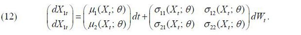
In order to account for the method of Aït-Sahalia (2008) briefly for a general two-dimensional model, let us look at a two-dimensional diffusion process Xt = (X1t, X2t)',
A diffusion process is said to be reducible if it can be transformed into a unit diffusion whose volatility function is the identity matrix. If a diffusion model is reducible, an approximate log-likelihood function can be derived explicitly using the Hermite expansion or the Kolmogorov method. Aït-Sahalia (2008) and Choi (2013) present additional details of the reducible method. To determine if model (12) is reducible, it suffices to check the following necessary and sufficient conditions for a two-dimensional diffusion process,
where  , i = 1, 2 is the (i, j) element of the inverse matrix of the volatility σ(x; θ) in (12). However, when checking these equalities for the Heston, GARCH, and CEV
models, none of them are found to be reducible. In this case, although the reducible
method is not applicable, the irreducible method can be adopted to obtain a closed-form
approximate log-likelihood function. The irreducible method is more general than the
reducible method, and it can be applied to any multivariate diffusion process, roughly
speaking, as long as it has differentiable drift and volatility functions.
, i = 1, 2 is the (i, j) element of the inverse matrix of the volatility σ(x; θ) in (12). However, when checking these equalities for the Heston, GARCH, and CEV
models, none of them are found to be reducible. In this case, although the reducible
method is not applicable, the irreducible method can be adopted to obtain a closed-form
approximate log-likelihood function. The irreducible method is more general than the
reducible method, and it can be applied to any multivariate diffusion process, roughly
speaking, as long as it has differentiable drift and volatility functions.
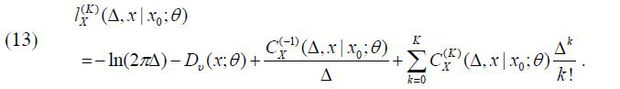
The starting point when deriving an approximate log-likelihood function employing the irreducible method is to surmise the functional form as that acquired for reducible diffusions:
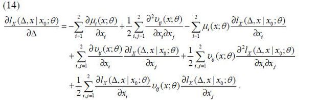
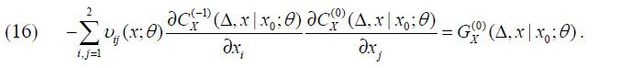
It is well known that the true log-likelihood function satisfies the Kolmogorov forward and backward partial differential equations (PDEs). The former is
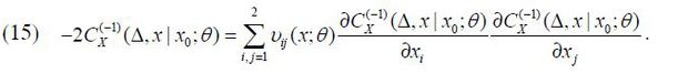
Therefore, if we substitute  for lx (Δ, x | x0; θ) in equation (14) and equate the same order terms of Δ, we can obtain the following
PDEs of the coefficients
for lx (Δ, x | x0; θ) in equation (14) and equate the same order terms of Δ, we can obtain the following
PDEs of the coefficients  , k ≥ −1.
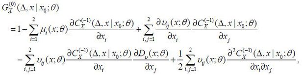
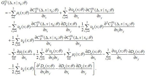
and for all k ≥ 1
where
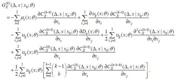
and when k ≥ 2
It is important to note that v(x; θ) = σ(x; θ)σ(x; θ)T and σ(x; θ)T is the transpose of σ(x; θ).
When Xt is reducible, the explicit solutions of the above PDEs of can be found (see Choi (2015a)). Alternatively, Xt can be transformed into a unit diffusion process with the findings in Aït-Sahalia (2008) then used to obtain the closed-form approximate log-likelihood function. However,
none of our models are reducible. Even so, we can turn to the irreducible method developed
by Aït-Sahalia (2008). The major idea of the irreducible method is to Taylor-expand each coefficient and all of the other functions of x around x0 in the above PDE. Subsequently, equating the same orders of (x − x0) yields an approximate coefficient of . The approximation order jk of is set to have an approximation error identical to Op(ΔK+1) of the approximate log-likelihood function. Specifically, jk = 2(K − k + 1), for instance, when k = 2, the orders of the Taylor expansion are j−1 = 8, j0 = 6, j1 = 4, and j2 = 2. We denote the jk -th order Taylor expansion of by  , k ≥ −1. The procedure of finding from the PDE of must be done from a low order to a high order recursively because the latter is generally
dependent on all of the low-order terms. Moreover, must be retrieved in sequence from k = −1 sequentially because the PDE of usually contains all of the previous terms.3 In this manner, we are able to obtain the approximate log-likelihood function up
to any order.4.
, k ≥ −1. The procedure of finding from the PDE of must be done from a low order to a high order recursively because the latter is generally
dependent on all of the low-order terms. Moreover, must be retrieved in sequence from k = −1 sequentially because the PDE of usually contains all of the previous terms.3 In this manner, we are able to obtain the approximate log-likelihood function up
to any order.4.
We have estimated the Heston, GARCH and CEV models presented in Section 3 using daily observations of the KOSPI 200 for stock prices and the integrated volatility as a volatility proxy constructed from the daily VKOSPI data for Korea. We also conducted the same estimation using the daily S&P 500 and the VIX for the US stock market to compare the Korean and US stock markets. The estimation results are displayed in Table 4. Note that the CEV model encompasses the other two stochastic volatility models, as noted above.
MLE was carried out with the approximate log-likelihood function obtained by applying the irreducible method. In doing so, β is found to converge to 0.5, which amounts to the Heston model for Korea. However, this does not arise in the case of the US stock market. Therefore, we do not report estimation results of the CEV model for Korea. Two information criteria, AIC and BIC,5 are reported in the last two rows of Table 4. Both AIC and BIC prefer the Heston model to the GARCH model for Korea because the Heston model has smaller AIC and BIC values than the GARCH model. On the other hand, the CEV model is selected by AIC and BIC, as the CEV process yields the smallest AIC and BIC values among the three models.
Note: Maximum likelihood estimation results of the Heston and GARCH models for Korea and the Heston, GARCH, and CEV models for the US are tabulated in this table. No estimation results are given for the CEV model of Korea because the CEV model converges to the Heston model for the Korean data. The last three rows display the maximized log-likelihood, AIC and BIC values for each case. The two asterisks by each estimate imply statistical significance at the 1% level. From the second column to the seventh column, the estimation results for the Heston and GARCH models for Korea and for the Heston, GARCH and CEV models for the US are correspondingly presented.
The parameter ρ measures the correlation between the logarithm of the stock price and the integrated
volatility proxy. For the Heston process of the Korean stock market, the estimate
of ρ is −0.61 and is statistically different from zero at the 1% level. We also obtained
similar results for p in the GARCH model. These estimates are quite analogues to the
sample correlation between the ln(KOSPI 200) and IV, which shows that there exists a strong leverage effect in the Korean
stock market. Like the Korean stock market, the US stock market also appears to have
a leverage effect. From the CEV model, we found that  , statistically significant at the 1% level, while
  and −0.70 for the Heston and GARCH processes, respectively. For the US, the CEV model
engendered an estimate of the leverage effect of −0.64, much closer to the sample
correlation between the ln(S & P 500) and the IV as compared to the other two nested models.
and −0.70 for the Heston and GARCH processes, respectively. For the US, the CEV model
engendered an estimate of the leverage effect of −0.64, much closer to the sample
correlation between the ln(S & P 500) and the IV as compared to the other two nested models.
The speed of reverting to the long-run mean level of the IV is very accurately estimated to be 6.09 for the Heston model, while it is 6.93 for the GARCH model for Korea. For the US stock market, the estimate of κ is 5.50 for the CEV process and 2.85 and 2.59 for the other two models, correspondingly. All estimates of κ are statistically greater than zero at the 1% significant level. The volatility of the Korean stock market has been found to revert to its long-run mean more rapidly than that of the US stock market. Computing the expected time6 it takes for the IV process to return to the middle value between the current value of IV and the longrun mean level of the IV based on the estimate of κ from the best model for each country, it is 28.68 business days for Korea and 31.76 business days for the US.
Even if we obtained statistically significant estimates of the speed of mean reversion for all cases, none of the long-run mean levels γ are statistically significant. Even so, the estimate of γ of the preferred model for each country, the Heston model for Korea and the CEV model for the US, is similar to the sample mean of the integrated volatility proxy variable. Figures 5 and 6 draw these estimates of γ with the integrated volatility proxy values during the data period for Korea and the US. It appears to be reasonable to contend that the IV reverts to the estimated long-run mean value for both countries. We did not obtain a statistically significant estimate of γ most likely because there may be more than one data-generating process depending on the state of the economy. Using a regime-switching model, we may be able to attain statistically more significant estimates of γ, as found by Choi and Yuan (2018) for the US. It can be interesting to determine if there is more than one regime and, if so, how the estimates of the long-run mean and mean reversion speed differ in different regimes for the Korean stock market. This is left as future research.
DAILY OBSERVATIONS OF THE INTEGRATED VOLATILITY AND  FOR THE HESTON MODEL OF KOREA
Note: Figure 5 draws a daily time-series plot of the integrated volatility proxy of Korea. The horizontal line is the estimated long-run average from the Heston model.
DAILY OBSERVATIONS OF THE INTEGRATED VOLATILITY AND FOR THE CEV MODEL OF THE US
Note: Figure 6 draws a daily time-series plot of the integrated volatility proxy of the US. The horizontal line is the estimated long-run average from the CEV model.
Like the parameter γ , no significant estimate of r − d was obtained for any of the models for any country.7 The market price of risk for the stock price variable has been estimated to be significant in all cases. For Korea, these values are 3.95 and 4.42 for the Heston and GARCH models, respectively. In the case of the US, they are 4.94, 4.42 and 3.00 respectively for the Heston, GARCH, and CEV processes. Using the best model for each country, the market price of risk for the stock price is found to be more expensive in Korea.
Finally, looking at the parameters associated with the volatility function of the integrated volatility proxy, all of them are statistically greater than zero. In fact, it is more informative to draw and compare the volatility functions of the IV. Figure 7 depicts the volatility functions evaluated at the ML estimates with their 95% confidence bands over the range of the observed integrated volatility proxy for each country. The GARCH process underestimates (overestimates) the volatility of the IV when the IV is small (large), as indicated in the left panel of Figure 7 given the evidence that the Heston model is preferred to the GARCH model in Korea. The CEV model is better than the other two models and the Heston and GARCH processes overestimate the volatility of the IV for all observed values. Contrasting the Heston model of Korea and the CEV model of the US, the IV is more volatile in Korea than in the US for the entire range of the IV.
Note: The panel on the left and that on the right in Figure 7 depict the volatility functions of the integrated volatility proxy of Korea and the US, respectively. The volatility functions of the IV in the Heston and GARCH processes for Korea and those in the Heston, GARCH and CEV processes for the US are evaluated at the maximum likelihood estimates over the range of the IV observed. The dotted lines are 95% confidence bands.
We have found that most estimates of the parameters of the stochastic volatility models examined here are quite accurate for both stock markets. Furthermore, stochastic volatility models can capture well-known characteristics of share prices in both countries. This implies that introducing another stochastic factor for the instantaneous volatility of the stock price is desirable to fit the data better for both Korea and the US. Therefore, the stochastic volatility model appears to be more appropriate than the Black-Scholes-Merton model in explaining the movements of stock prices at least for these two countries.
This article estimates the three continuous-time stochastic volatility models of the Heston, GARCH, and CEV models using daily data from KOSPI 200 and the VKOSPI for Korea and daily observations of the S&P 500 Index and the VIX for the US. We generate an integrated volatility proxy for an unobserved volatility variable using the implied volatility of an at-the-money option maturing in 30 calendar days. The VKOSPI and the VIX are the implied volatilities employed, respectively, for the Korean and US stock prices. MLE is utilized to estimate the parameters of these three models. To do this, we need the transition probability density functions (TPDFs) of our diffusion processes. However, the true TPDFs are not known for any of our models. Therefore, we adopt the irreducible method suggested by Aït-Sahalia (2008) to approximate the TPDF in a closed form accurately.
We were able to identify well-known features of stock prices in both countries. The Heston model and the CEV model are found to be best among the three models for the Korean and US stock markets, respectively, according to the information criteria, AIC and BIC. From the estimation results, we find that there are relatively strong leverage effects in both countries. The long-run mean level of the integrated volatility proxy (IV) was not statistically significant in either market. This appears to be due to the fact that we attempt to fit the data using only one data-generating process. It may be more reasonable to contend that stock prices are governed by more than one data-generating process depending on the economic weather. The CEV model converges to the Heston model for Korean stock prices possibly for the same reason. The speeds of mean reversion parameters are statistically significant in both markets. The IV is found to return to its long-run mean value more rapidly in Korea than in the US. All parameters related to the volatility function of the IV are statistically significant. The elasticity of the volatility of the IV is 0.50 for Korea and 0.62 in the US. Although it is more elastic in the US stock market, the volatility itself is greater in Korea than in the US over the range of observed IV outcomes. The mean-reversion speed and the volatility of the IV may vary depending on the economic conditions. If we allow the parameters to change over time, we may be able to obtain more interesting results. Choi and Yuan (2018) found strong evidence of regime-switching in the US stock market. It would be valuable to investigate Korean stock markets using regime-switching stochastic volatility models, which is an ongoing research topic.
Finally, we found evidence that there exists a strong leverage effect in both countries. This means that investors who buy stocks on margin are more likely to suffer large losses, particularly when the stock market is in a downturn. Therefore, in order to stabilize the stock market, it appears to be necessary for policymakers to prohibit excessive purchases of stocks on credit.
I am very grateful to the Editor, Professor Siwook Lee and two anonymous reviewers for their valuable comments and suggestions, which helped me to improve this article considerably. This work was supported by the 2017 sabbatical year research grant of the University of Seoul.
We could use (VIXt / 100)2 and (VKOSPIt / 100)2 as proxies of the true instantaneous volatility state variables for the US and Korea,
respectively. However, as Aït-Sahalia and Kimmel (2007) argue, using these unadjusted Black-Scholes proxies introduces significant bias in
the estimation of the elasticity of volatility parameter for the more general CEV
model. They remedy this by correcting for the effect of the mean reversion of the
volatility and provide equation (1) to calculate the integrated volatility proxy,
IVt from unadjusted BlackScholes proxy, . In doing so, we need a and b in equation (1), which are estimated from equation (2).
Because model (2) is univariate and reducible, the reducible method can be used to find the approximate TPDF. To use the reducible method, however, we need to consider three different cases, where 0 < β < 1, β = 1 and β > 1 , and find the approximate TPDF for each case, which can be cumbersome. See Aït-Sahalia (1999) for more on this. Instead, if we use the irreducible method, we do not have to take these three cases into account separately.
The Kolmogorov backward partial differential equation for the log-likelihood function
of Xt is  Employing the backward PDE instead of the forward PDE, we obtain the PDEs of the
coefficients in x0 and Δ. Using those PDEs of
Employing the backward PDE instead of the forward PDE, we obtain the PDEs of the
coefficients in x0 and Δ. Using those PDEs of  , the same Taylor expansions of the coefficients can be retrieved. Thus, which PDE
is used is irrelevant.
, the same Taylor expansions of the coefficients can be retrieved. Thus, which PDE
is used is irrelevant.
We can also obtain an approximate transition probability density function. Choi (2015b) presents more information about how to obtain the approximate transition probability density function from the approximate loglikelihood function.
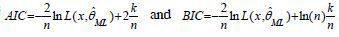 , where n is the number of observations minus one and k is the number of parameters for each model. In addition,
  is the likelihood value evaluated at the maximum likelihood estimates.
The amount of expected time it takes for a mean-reverting process to revert halfway back to the long-run mean value is termed the half-life. For a diffusion process with a linear drift function κ(Xt − γ), the half-life is ln(2) / κ. Because we use daily observations, the number of half-life days can be calculated as 252·ln(2) / κ.
Aït-Sahalia and Kimmel (2007) did not estimate this parameter. In fact, the instantaneous interest rate and dividend yield for stocks were held fixed at 4% and 1.5% per year, respectively.
(1999). Transition Densities for Interest Rate and Other Nonlinear Diffusions. Journal of Finance, 54, 1361-1395, https://doi.org/10.1111/0022-1082.00149.
(2002). Maximum Likelihood Estimation of Discretely Sampled Diffusions: A Closed-Form Approximation Approach. Econometrica, 70(1), 223-262, https://doi.org/10.1111/1468-0262.00274.
(2008). Closed-Form Likelihood Expansions for Multivariate Diffusions. Annals of Statistics, 36(2), 906-937, https://doi.org/10.1214/009053607000000622.
, & (2007). Maximum likelihood estimation of stochastic volatility models. Journal of Financial Economics, 83, 413-452, https://doi.org/10.1016/j.jfineco.2005.10.006.
, & (1998). Nonparametric estimation of state-price-densities implicit in financial asset prices. Journal of Finance, 53, 499-547, https://doi.org/10.1111/0022-1082.215228.
, , & (2006). Estimation of Continuous-time Models with an Application to Equity Volatility. Journal of Financial Economics, 82, 227-249, https://doi.org/10.1016/j.jfineco.2005.09.005.
, & (1973). The Pricing of Options and Corporate Liabilities. Journal of Political Economy, 81, 637-654, https://doi.org/10.1086/260062.
, & (2003). Spectral GMM Estimation of Continuous-Time Processes. Journal of Econometrics, 116, 259-292, https://doi.org/10.1016/S0304-4076(03)00109-X.
, , & (1992). An Empirical Comparison of Alternative Models of the Short-Term Interest Rate. The Journal of Finance, 47(3), 1209-1227, https://doi.org/10.1111/j.1540-6261.1992.tb04011.x.
, & (2011). On the Approximate Maximum Likelihood Estimation for Diffusion Processes. Annals of Statistics, 39(6), 2820-2851, https://doi.org/10.1214/11-AOS922.
, , & (2015). An Asymmetric Nature of the VKOSPI Index. The Journal of Eurasian Studies, 12(4), 21-43, https://doi.org/10.31203/aepa.2015.12.4.002.
(2013). Closed-Form Likelihood Expansions for Multivariate Time- Inhomogeneous Diffusions. Journal of Econometrics, 174(2), 45-65, https://doi.org/10.1016/j.jeconom.2011.12.007.
(2015b). Explicit Form of Approximate Transition Probability Density Functions of Diffusion Processes. Journal of Econometrics, 187, 57-73, https://doi.org/10.1016/j.jeconom.2015.02.003.
, , & (2003). Maximum Likelihood Estimation of Time Inhomogeneous Diffusions. Journal of Econometrics, 114, 107-139, https://doi.org/10.1016/S0304-4076(02)00221-X.
(1952). The Parabolic Differential Equations and the Associated Semi-Groups of Transformations. Annals of Mathematics, 55(3), 468-519, https://doi.org/10.2307/1969644.
(1993). A Closed-Form Solution for Options with Stochastic Volatility with Applications to Bond and Currency Options. Review of Financial Studies, 6(2), 327-343, https://doi.org/10.1093/rfs/6.2.327.
, & (1987). The pricing of options on assets with stochastic volatilities. Journal of Finance, 42, 281-300, https://doi.org/10.1111/j.1540-6261.1987.tb02568.x.
(2003). The dynamics of stochastic volatility: evidence from underlying and options markets. Journal of Econometrics, 116, 181-224, https://doi.org/10.1016/S0304-4076(03)00107-6.
(2010). A damped diffusion framework for financial modeling and closed-form maximum likelihood estimation. Journal of Economic Dynamics and Central, 34, 132-157, https://doi.org/10.1016/j.jedc.2009.08.001.
(1973). Theory of Rational Option Pricing. Bell Journal of Economics and Management Science, 4, 141-183, https://doi.org/10.2307/3003143.
(1990). ARCH models as diffusion approximations. Journal of Econometrics, 45, 7-38, https://doi.org/10.1016/0304-4076(90)90092-8.
, & (1991). Stock Price Distributions with Stochastic Volatility: An Analytic Approach. Review of Financial Studies, 4, 727-752, https://doi.org/10.1093/rfs/4.4.727.
(1989). Overreactions in the options market. Journal of Finance, 44, 1011-1023, https://doi.org/10.1111/j.1540-6261.1989.tb02635.x.
, , & (2010). Bayesian Inference for Discretely Sampled Markov Processes with Closed-Form Likelihood Expansions. Journal of Financial Econometrics, 8(4), 450-480, https://doi.org/10.1093/jjfinec/nbp027.
(2007). Closed-Form Likelihood Approximation and Estimation of Jump-Diffusions with an Application to the Realignment Risk of the Chinese Yuan. Journal of Econometrics, 141, 1245-1280, https://doi.org/10.1016/j.jeconom.2007.02.003.