Analysis on Korean Economy with an Estimated DSGE Model after 2000

1. Households Problem

There is a continuum of households in the economy index by j which maximizes the lifetime utility function over consumption, real money balance and leisure.

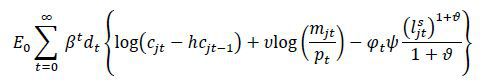
where ݄h is the habit persistence and ϑ is Frisch labor supply elasticity. Habit formation for consumption generates hump-shaped response of consumption to stochastic disturbances. And thus this creates another smoothing mechanism of consumption path on the top of smoothing due to log-utility. The separable utility for real money balance does not play a qualitative role to change other real allocations since the monetary policy is implemented via open market operation rather than money printing but only to be included in the government budget constraints. ݀d_t is an intertemporal preference shock and φ_t is a labor supply (or intertemporal) shock :

Those preference shocks will act as aggregate demand shocks in the economy. The intertemporal shock, d_t, is an important source of business cycle fluctuations according to Primiceri et al. (2006). And the labor supply shock, φ_t, stands for changes in employment that is another source of aggregate fluctuations.11

The j^th household’s budget constraint is given by :

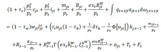
p_t is price level of final domestic good which is numerarie in this model. and are prices of final consumption and investment good that differ from p_t since they are composites of final domestic and final imported goods. B_jt is nominal domestic bond holding with uncontingent gross interest rate, R_t, and a_jt+1 is Arrow contingent bond for every state which forms a complete asset market within the economy.

In the international asset market, however, household can only purchase uncontingent foreign bond, ex_t, where is in foreign currency and ex_t is the exchange rate. The world interest rate associated with this foreign bond evolves as

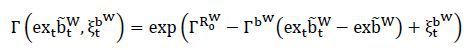
Since the risk free interest rates of Korea has shown difference from world interest rate such as U.S. Treasury Bill, the world interest rate cannot directly be the price of foreign bond which the household must bear. Thus, the country risk premium is included to the gross interest rate of foreign bond by Γ(⋅) for possible time variation and systematic gap. In order to close the small open economy, i.e. to prevent from nonstationary responses of variables to world interest rate shock, as argued by Schmitt-Grohé and Uribe (2003), the risk premium is modeled as debt elastic. The functional form for premium is

where time varying premium shock

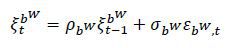
and the share of foreign bond holdings as

is the systematic gap that implies the average interest rate spread between the Korean interest rate and the world interest rate. The term, , ensures the foreign debt does not explode by penalizing the risk premium when foreign debt is increased.

w_jt is the real wage from the differentiated labor supply, . r_t is the rental price of capital, u_jt > 0 is the intensity of use of capital, and Φ[u_jt] is the physical cost12 of use of capital in resource term where

μ_t is an investment-specific technology shock or also its inverse is interpreted as the relative price of investment good in final good unit. As mentioned earlier, this can capture the gap between investment time series and output. Since the Korean investment growth has been lower than any other GDP components, it is likely to have negative trend in this process during the sample period. The exogenous process is

And the capital stock13 evolves with

where

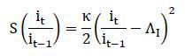
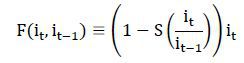
S(⋅) is the investment adjustment cost which is a smoothing mechanism for investment and thus generates hump-shaped response to shocks, if not, the implied investment becomes too volatile. Due to this cost, Tobin’s Q, q_t, which is the price of installed capital becomes time varying. For ease of notation, define

and

There are three types of taxes on consumption, wages and capital income. Note that the tax on capital income is only for the net return of capital after depreciation and thus the tax credit, δτ_k, is included.

Symmetric Equilibrium Since we consider a symmetric equilibrium due to complete asset market (the complete set of state contingent Arrow securities and perfect risk sharing) so that c_jt = c_t, B_jt = B_t, = , λ_jt = λ_t, u_jt = u_t, q_jt = q_t, i_jt = i_t, k_jt = k_t except for the wage and differentiated labor supply. After rearranging FOCs from household optimization problem,

Household Labor Problem The labor problem for the household can be solved separately due to the separable utility. The household who is allowed to optimize with a probability, θ^w, its wage maximizes the possible future stream of wage revenues when the wage is not allowed to be optimized minus its future stream of disutilities from labor supply. The household posts its monopolistic competitive wage and its labor supply is determined via labor demand function which is derived from the labor packer’s problem.14 η is the elasticity of substitution between differentiated labors, and the following demand function is a standard outcome from Dixit-Stiglitz type of aggregation of differentiated labors in a monopolistic competitive market. Also, to generate a possible persistence for the inflation of wage a partial indexation, parameterized by χ_w, is adopted. In summary, the household maximizes net revenue in utility terms with respect to its wage subject to labor demand function.

subject to

The FOCs of this problem will yield an optimal wage level by equilibrating the intertemporal marginal revenues to intertemporal marginal disutilities. Those households who allowed to optimize at t will set the same wage level due to the perfect risk hedging for the timing of wage change. Thus, the optimal conditions in this problem becomes symmetric. Now, these conditions can be better implemented in computation if it is transformed into recursive representation by introducing an auxiliary variable, f_t. After a tedious algebra, the law of motion for the recursive representation becomes

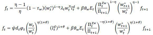
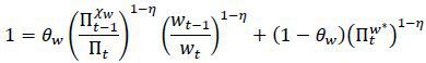
where is the symmetric optimized real wage for households who are allowed to optimize while w_t is the aggregate real wage for all households. Since in Calvo-Yun setting, there is a fixed population of households who are allowed to set wage with 1 − θ^w and who are not with θ^w, the real wage index evolution can be derived by aggregation.

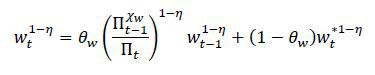
which can be rewritten

where

2. The Distribution Sector

A. Final Consumption and Investment Good Producers

Perfectly competitive final consumption good producer and investment good producer pack domestic consumption and investment good (, ) with imported consumption and investment good (, ) to produce final consumption and investment good (c_t, i_t) using following CES technology :

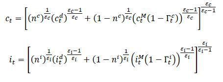
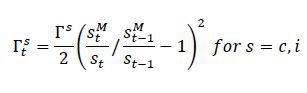
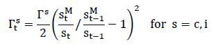
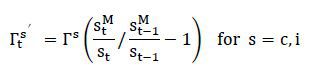
where home biases, n^c and nⁱ, are present. ε_c and ε_i represent elasticity of substitution between domestic and imported good. In order to dampen the excessive volatility of imported goods that affects the final consumption and investment, a costly transformation of imported goods in the aggregation technology is adopted.15 The cost function is a quadratic form of a growth rate of a share of imported good. The cost function for this is denoted by and where

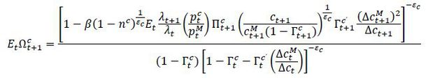
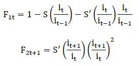
Due to this adjustment costs that depends on the past share of imported goods, the problem for final good producer becomes dynamic instead of a standard static problem.16 :

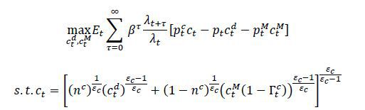
Solving this problem, the equilibrium conditions are :

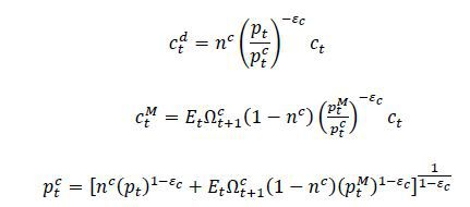
where

B. Final Domestic Good Producer

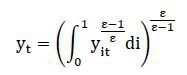
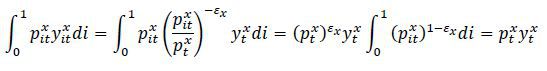
Final domestic good producer produces a homogenous final good to sell at a perfectly competitive market using intermediate good with the Dixit-Stiglitz technology.

where ε is the elasticity of substitution between intermediated goods. The static problem of the final good producer is

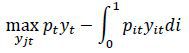
subject to

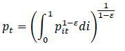
gives input demand function

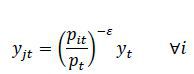
where the aggregate price level is

The problems for the labor packer, imported goods distributor and foreign importers who purchase domestic exported goods are all similar to this final good producer’s problem in which demand functions for differentiated goods are derived. Henceforth, demand functions directly appear as constraints to differentiated goods producers without solving each problem.

C. Intermediate Good Producers

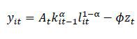
There exists a continuum of intermediate good producers whose i^th firm’s technology is

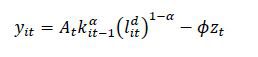
where k_it and l_it are capital services and homogenous labor. ϕ is fixed cost parameter to guarantee zero profits in the economy at steady state (No entry or exit).

And

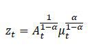
Now, A_t follows

A_t = A_t-1exp(logΛ_A + σ_Aε_A,t)

This exogenous process is a total factor productivity with a trend. The trend in this process together with the investment specific trend constitutes a balanced growth path of the economy. This outcome of these two trends is only possible due to a particular functional form of the production technology which is Cobb-Douglas. First, define μ_A,t ≡ then, we can rewrite

log μ_A,t = logΛ_A + σ_Aε_A,t

and define , then

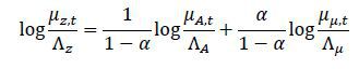
where

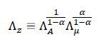
This weighted average of trends will be used to stationarize the system.17

The problem for intermediate good producer can be dissected into two stage. First problem is a static cost minimization where the firm decides how much to employ labor and capital from perfectly competitive factor markets. The other problem is a price setting under Calvo-Yun friction which becomes dynamic.

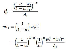
Factor Demands Firm pays wage and rents, w_t and r_t, for and k_it-1. The firm solves a static cost minimization problem,

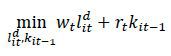
subject to the production

Assuming interior solution, FOCs are

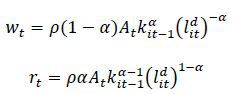
where ρ is the Lagrangian multiplier. The capital labor ratio is derived from above two equations,

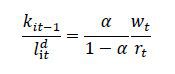
This implies capital labor ratio is same across the intermediate good producing industry and thus real marginal cost is also same. We can find real marginal cost mc_t by setting 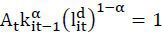. This implies

Price Setting Calvo-Yun pricing decision is similar to wage setting problem from the previous section only to replace marginal revenues and marginal costs. Since the firm is owned by households, the firm discounts the future stream of profits from households’ point of view and thus by the stochastic discount factor. A partial indexation is again introduced and so the firm sets the price to maximize :

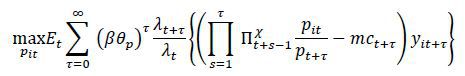
subject to

Similarly, the law of motion can be summarized by

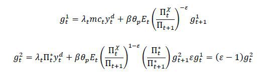
where . Due to fixed population of firms who optimize price and who cannot, the aggregate price level evolves as

3. Foreign Sector

The demand functions in the foreign sector are shown first and price setting problems in the foreign sector appear later in this subsection.

A. Importing Firms

The distributor produces the final imported good from differentiated imported goods by aggregation with following technology :

where ε_M is the elasticity of substitution across foreign imported goods. The import demand function and the price of the imported final good are,

The total amount of imported goods is given by:

B. Exporting Firms

There exists a continuum of monopolistically competitive exporting firms who buy the final domestic good and differentiate it by brand naming. They sell those goods to importers from the rest of the world. Each exporting firm faces following demand function :

where both prices are expressed in the foreign currency of the export market. The export price is

And the total amount of exported good is given by :

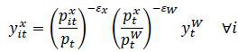
And since the economy is a small open economy with measure zero, we can safely assume that the world demand for our export is,

Thus combining above demand functions gives,

The world demand is exogenously given by :

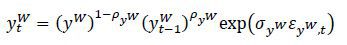
and world inflation, , by :

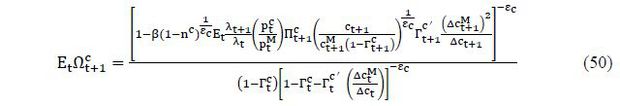
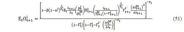
C. Price-setting in the Foreign Sector

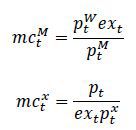
Calvo-Yun price setting for importing and exporting firms is assumed to allow for incomplete exchange rate pass through. The problem of importing and exporting firms is identical and thus,

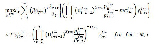
where the real marginal costs in domestic and foreign currency terms for importing and exporting firms are,

Similar to imtermediate domestic good producers, price setting equilibrium conditions in recursive forms for importing and exporting fimrs can be derived as :

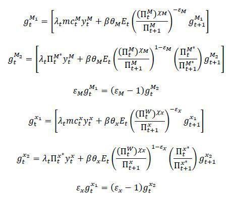
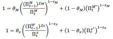
where and Price evolution for import and export goods is,

D. Evolution of Net Foreign Assets

The balance of payments which binds the current account and capital account together evolves as follows :

where we have used the fact that :

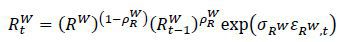
4. Monetary Authority

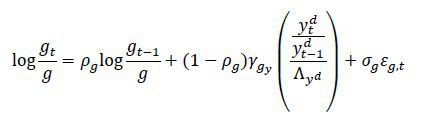
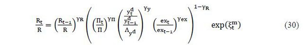
While the monetary authority’s primary goal is to stabilize the inflation, output stability can be another important objective. Thus, an augmented Taylor rule in which the interest rate not only responds to inflation gap but also to output gap is generally assumed. In addition, the growth rate of the exchange rate is added to reflect more realistic setting for a small open economy like Korea who in practice wants to stabilize the exchange rate as well. The monetary authority sets the nominal interest rates according to :

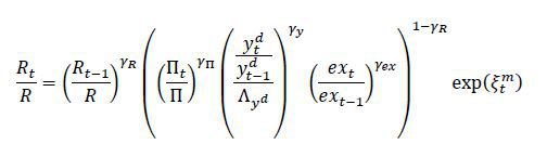
Π represents the target level of inflation (equal to inflation trend in the steady state in this model), R steady state gross return of asset, and Λ_y^d the steady state gross growth rate of . The term is a random shock to monetary policy that follows .

5. Government

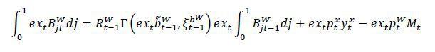
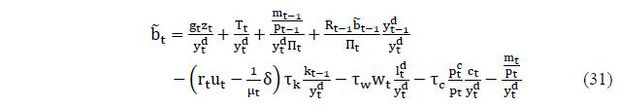
The government’s revenues are generated by marginal taxes and lumpsum tax (or negative lumpsum subsidy) while the expenditures are determined with an exogenous shock and an automatic stabilizer. The government budget constraint is :

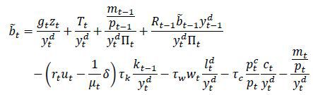
where . The real government expenditure is exogenously given by,

But level of debt should be prevented from exploding and thus the lumpsum transfer should be designed to be controlled by the deviation of debt from its own steady state level

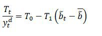
where the steady state of debt level

1. Data

<Table 6>

Data Source

Domestic data are imported from ECOS (Economic Statistics System of the Bank of Korea) and KOSIS (Korean Statistical Information Service) while foreign data are from FRED and Global Insight. The model described in this paper is a practically representative agent model so that the variables of interest such as output and expenditures are in terms of capita. As KOSIS only provides annual data for population, the quarterly time series was constructed by a linear interpolation to divide GDP components. Another indirect mapping from the raw data to the model is applied with private consumption, private investment and government expenditures. Durable consumption is excluded from private consumption variable in the model but is instead included in the private investment. This treatment can be done in practice when the model does not specify durable goods sector explicitly since the utility flow from consuming durable goods is not concentrated in one decision time period but dissembled for prolonged periods. Also, durable goods are generally depreciated over periods which show more of an investment characteristic in the model. Hence, the private consumption is constructed by nondurables, semidurables and services while the private investment is constructed by durables and private fixed capital formation. Government expenditures are constructed based on addition of government consumption and government fixed capital formation as they are not reported in KOSIS. As noted earlier in section II, KOSIS GDP components in real terms are based on Lespeyres chain weighted index. Having this taken into account, the constructed series are recovered.18 The consumption deflator associated with this constructed consumption is computed as byproduct to be used for estimation.

Although Call rate is the policy rate for the Bank of Korea, the risk free interest rate in this paper not only represents the policy rate but also the interest rate which households directly face at the same time without risk premium or financial friction. Hence, 1 year Treasury Bond rate was chosen to serve as proxy for the risk free domestic interest rate. And the world interest rate is 3 months U.S. Treasury Bill. For labor supply, total working hours from raw data is normalized so that it is between zero and one. DSGE models in general are hard to replicate the excessive volatilities of the nominal exchange rates. Nevertheless, Won/Dollar exchange rate has been included in the dataset because of the inclusion of the global financial crisis in 2008. The export for Korea in Won during 2008 has exceeded the growth of world demand. This cannot be explained either by the world demand or the world inflation both of which have been decreasing during the crisis. It is only possible with a strong depreciation of Korean Won. The proxy for the world inflation is the deflator for the sum of GDPs of 11 major trading partners with Korea. As it was motivated in section II, the World Trade Volume is chosen for world demand in the model. It is worth noting that the World Trade Volume is a nominal value in terms of the U.S. dollars. So the variable from the model should be constructed accordingly.

GDP components and World Trade Volume are transformed into growth rates for stationarity.

In summary, there are twelve time series data available for the estimation; domestic interest rate, inflation rate of consumption deflator, labor hours, GDP, private consumption, private investment, government expenditures, exports, world demand, world interest rate, world inflation and exchange rate. So the observable vector in log-deviation from steady state is,

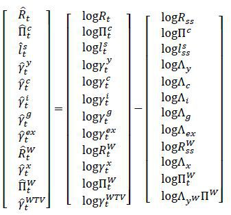
where Λ_z = Λ_y = Λ_c = Λ_g = Λ_x = Λ_yw , Λ_ex = 1 , Π^C = Π^W and R_SS =

But using all of those time series have not necessarily resulted in good fit of key macro variables as shown below. Thus, we present the various results with different combinations of selected time series after econometric methodology subsection. The key variables that were included with any set of observables were domestic interest rate, domestic inflation rate, labor hours, GDP, consumption, investment, government expenditures, exchange rate and world interest rate. Three variables from world demand, world inflation rate and exports were brought to test different sets of combinations. In order to avoid the stochastic singularity problem and also to minimize any excessive movements of observables, measurement errors have been specified when the model is brought to the estimation with 10% of each own variabilities in observations except for the exchange rate volatilities. The standard deviation of measurement error for the exchange rate growth is set as 35% of its own standard deviation in data. Although, this magnitude of standard deviation in measurement error is larger than other variables, this was necessary in order to derive reasonable magnitude of implied volatilities of other key macro variables. This limitation of empirical results is not alone since the volatility of exchange rate in general is difficult to be replicated in the context of sticky price DSGE models as argued by Chari et al. (2002). Nevertheless, the exchange rate growth has been included to explain the high growth of exports in Korean won during the global financial crisis. Otherwise, the model which estimated without the exchange rate growth19 was attributed the high growth of export in 2008 to the high world inflation which is inconsistent to our general understanding of the crisis periods.

2. Econometric Methodology

Bayesian method20 is adopted to map the data to the model. To make it implementable for estimation and various simulation exercises, the system of stationarized equilibrium conditions is approximated up to first order around the deterministic steady state. Since the posterior distribution of structural parameters is hard to be characterized analytically, Random Walk Metropolis-Hasting algorithm is used for the numerical approach. The proposal density is Hessian of the likelihood function evaluated at the posterior mode which is estimated via CMAES method.21 The posterior distributions reported in the following subsection are based on the second half of 5 million draws from MCMC algorithm, i.e. discarding the first 2.5 million draws for the initial burn-in. The acceptance ratio was approximately 61.34 % which indicates appropriate property for estimation.

There are a small set of parameters that are calibrated rather than estimated because they are either hard to be identified with macro time series or irrelevant, shown in <Table 7>. β is calibrated to match the steady state of Euler equation, . 22 The steady state condition requires β = . For calibration, sample mean of inflation, growth rate of output and interest rates are used for Π_SS , Λ_Z and R_SS . These values imply β of 1.0044 which seems unconventional. However, because the model has a balanced growth term, , β needs not to be less than one as long as 23 is less than one. With this calibrated β , the model is still stationary to any kind of shocks. is calibrated to match average total government debt to GDP ratio during the sample period as well as for to average nominal government to nominal GDP ratio. Besides being stationary in data, the other reason for calibrating the ratio instead of the level of government expenditures, ݃g, is that it allows us to solve the steady states of all the endogenous variables in closed forms. Otherwise, having ݃g calibrated would render a nonlinear equation for the labor supply to be solved.24 Marginal tax rates are calibrated to effective value-added tax revenues over private consumption, effective income tax over total wage income and corporate tax revenues over private capital formation. The rest of parameters are generally known to be standard in the class of DSGE models.

<Table 7>

Fixed Parameters

3. Empirical Moments of Estimated Models

Before the detailed results of the benchmark estimation are presented, first and second moments of the estimated models with different combinations of time series are reported in this subsection. There are seven possible estimations to choose from any combination of the last three observables. As <Table 8> shows, Model 1 estimates the model with first ten observables excluding the world trade volume and export growth, Model 2 excluding export growth and so on. The numbers in parenthesis are implied first moments of variables that were not included as observables in estimations. First moments implied by the estimated models do not show much differences across estimations since the long run trends’ estimates are mostly influenced by tight prior distributions. Note that the growth rates of GDP, consumption, government expenditures and exports are consistent within a model because they share the same balanced growth path by construction. However, this reason made the trends in world trade volume and export become difficult to match with data.

<Table 8>

First Moments

<Table 9> shows the volatilities of fitted observables. The fitted observables were estimated via smoothing Kalman Filter which retrieves the historical structural shocks. This procedure is generally done when it is necessary to demonstrate how the estimated DSGE model fits the data well. Thus, gaps between the actual observed data and the fitted values of observables have been filled by measurement errors. As can be seen from <Table 9>, the estimated models generally fit well with the data except the exchange rate growth. As mentioned earlier, this comes from the large magnitude of measurement errors which have been set intentionally for exchange rates.

<Table 9>

Volatilities of Fitted Observables

Another way of evaluating the empirical properties of estimated models is to observe the volatilities of simulated series. Table 1 shows the volatilities of observables simulated for the sample period. Given the estimated values for predetermined states25 in 2000:Q2 where the sample begins, the models are simulated onward until 2012:Q4 where the sample ends with randomly generating structural shocks. This has been done 10,000 times for each estimated model and averages over 10,000 standard deviations of simulated series which are collected in <Table 10>. In general, comparing the size of volatilities of each model to data shows that Model 1 and Model 3 match well at least with the observables. However, the implied volatilities of world trade volume and exports in Model 1 show significant discrepancy with data. On the other hand, Model 3 performs quite better even with matching the implied volatilities of unobservables to those of data. Therefore, we chose Model 3’s result as a benchmark estimation to be used for presenting detailed results below.

<Table 10>

Volatilities of Simulated Observables

4. Estimation Results

The prior and posterior distributions are reported in <Table 11>. There are several things worth noting with these estimates. First, the prior distributions are set as loosely as possible to meet reasonably good statistical properties of the whole estimation and follow much of the convention in the literature except parameters related to the trends. As Del Negro and Schorfheide (2008) has argued, the priors for trends such as, Λ_μ, Λ_A, Π and , need to be tight around the sample mean of time series directly related to these parameters. As mentioned earlier, the lower trend in private investment resulted in negative trends in Λ_μ along with the posterior estimates. Total factor productivity trend, on the other hand, reports 0.653. The inflation trend, Π, is estimated to be 0.716 which in per annum is approximately 2.863% close to the target inflation rate of the Bank of Korea. The average risk free interest rate spread between Korea and U.S. is estimated to be 0.636% which if translated to per annum results approximately in 2.544%.

<Table 11>

Prior and Posterior Distributions

Second, the preference parameters are mostly within standard boundary of estimates found in literature. The habit persistence parameter, ݄h, shows a strong persistence which seems obvious since the private consumption is defined as consumption of nondurables, semidurables and services. The inverse of Frisch elasticity, ϑ,was estimated to be 0.049 which is considerably lower than that of the U.S. and most of the developed countries.

Third, elasticities of substitutions vary across different sectors. The markups, − 1, implied by the estimates for domestic, imported and exported goods are 12.8%, 12.2% and 11.6%, respectively. This is not a surprising outcome since the Korean export sector faces more competitions in the world market compared to that of the import sector which faces far less competition. On the other hand, the wage markup, − 1, shows an estimate of 16.5% which implies the rigidity of the Korean labor market. Calvo parameters related to those sectors indicate stickiness in price changes, especially in the domestic good, θ_p, and exported good sector, θ_x. On the other hand, the estimate for the wage stickiness, θ_w, is 0.101 which is significantly lower than the usual findings in developed countries. This result combined with the high wage markup implies that there are more changes in the wage settings while the labor suppliers have market power in terms of negotiation. The adjustment cost parameter for imported consumption good, Γ^c, shows a higher degree of adjustment cost than that for imported investment good, Γⁱ, which implies that imported investment goods will add relatively more volatility towards the final investment good than imported consumption goods to final consumption good. This can be understood with the characteristics of the Korean manufacturing industries which mostly import raw materials and intermediate goods to produce final manufactured goods. The home biases, n^c and nⁱ, also demonstrate reasonable estimates, 0.857 and 0.234. Although this result relies somewhat on the prior distributions, it is consistent with the fact that consumption, in general, has more weights on nontradables such as services while the investment good consists less of nontradables but more of imported goods like machineries and installations.

Fourth, Taylor rule parameters in this estimation are γ_R, γ_Π, γ_y and γ_ex. The interest rate smoothing, γ_R, shows strong persistence. The inflation stabilization stance, γ_Π, is estimated to be 1.583 which is close to the prior. However, the posterior standard deviation is tighter than the prior distributions which indicates the likelihood of supporting the inflation stabilizing monetary policy during the sample period on average. On the other hand, the output gap stabilization stance parameter, γ_y, shows close to the prior mean to a less degree than γ_Π. And γ_ex shows the somewhat positive response of the monetary policy to the nominal exchange rates.26 And lastly, the positive estimate of γ_gy, the automatic stabilizer in the government expenditure process, shows countercyclicality.

Lastly, the autoregressive parameters to the structural shocks mostly show quite a strong persistence. The intra-temporal preference shocks, world interest rate shock and world demand shock particularly shows strong persistence while the inter-temporal preference shock, the government shock, risk premium shock and world inflation shock somewhat less. The standard deviation parameters of structural shocks indicate that the inter-temporal shock is the most volatile, followed by the world demand shock, intra-temporal shock and government expenditure shock.

The properties of prior and posterior distributions can be confirmed with the following figures. The thin lines indicate priors while the thick lines indicate posteriors. When the thick line is formed far from the thin line or shows tighter boundary, it means the structural parameter estimate is more strongly supported by data. This can be found easily with parameters related to structural shocks because posterior distributions of those parameters demonstrate stationary distributions. Most of the structural parameters show good identifications that are well supported by data with the exception of few parameters such as Γ_c, Γ^bw, θ_M and ξ_M which shows unsatisfactory data support. Trend parameters whose priors were set intentionally tighter would obviously result in posterior distributions that are close to prior distributions. Policy parameters except for the interest rate smoothing, γ_R, show that priors matter as well. The elasticities, ε' s and η,show reasonably well boundedness although the mixing properties are somewhat less than ideal. In general, there is room for an improvement by letting the data tell much as it can but we believe this outcome of estimates show quite reasonable properties considering the relative shortage of samples of Korean data compared to other developed countries.

5. Model’s Properties

Next five following figures show impulse response functions of key variables to five different structural shocks. The variables are all in one hundred times of log deviations from steady states. A shock simulation is based on one standard deviation of posterior estimates. The variables are nominal interest rate, inflation rate of consumption deflator, output growth, consumption growth, investment growth, wage growth, labor hours, export growth, imported consumption, imported investment, import growth and nominal exchange growth, respectively from top left to bottom.

[Figure 4]

Prior & Posterior Distributions

[Figure 5] shows IRFs to inter-temporal preference shock. This shock brings today’s marginal utility relatively larger than tomorrow’s resulting in increased consumption at the expense of dissaving which in turn leads to less investment. But since the domestic output does not increase enough to meet the consumption demand, imported consumption good demand increases which entails increase in inflation and depreciation of Korean won.

[Figure 5]

IRFs to Inter-temporal Preference Shock

[Figure 6] is IRFs to total productivity shock. The results in this figure are consistent with the convention in RBC models. Thanks to an increase in total factor productivity, the output grows and household increases consumption but with smoothing over time by saving in the initial period. Marginal productivity of labor, which is practically close to the wage in this estimated model due to weak wage stickiness, increases. Since the interest rate does not move significantly at the initial period while prices drop, uncovered interest parity condition requires that the exchange rate decreases and which leads to an appreciation of Korean won.

[Figure 6]

IRFs to Total Productivity Shock

[Figure 7] is IRFs to expansionary monetary policy shock. When the interest rate decreases by approximately 25bp , i.e. expansionary, the real variables such as output, consumption, investment, wage and labor hours increase due to price stickiness. Those firms that produce intermediate goods that are unable to optimize the price can only adjust real allocations which means that change in nominal interest rate has propagation mechanism on real variables. Since inflation rate increases as much as in Neoclassical models, increase of output results largely from favorable investment opportunities with more imported investment goods. Fall in interest rate combined with rise in inflation rate also depreciates Korean won which is implied by uncovered interest parity.

[Figure 7]

IRFs to Monetary Policy Shock

[Figure 8] is IRFs to government expenditure shock. Although increase in government expenditure boosts up the output of the economy, this should be seen as a mere alteration in accounting record rather than having an expansionary effect on other domestic demands such as consumption and investment in a concrete manner. Decrease in consumption and investment is a clear sign of crowding out effect of expansionary government expenditure. Thus this model does not imply the effectiveness of government expenditure policy on private sectors of the economy as it focuses rather on sticky price features

[Figure 8]

IRFs to Government Expenditure Shock

Lastly, [Figure 9] shows IRFs to the world demand shock. World demand first influences the export growth which leads to more demand in domestic productions from abroad. This raises the prospects of domestic firms and thus increases investment. Consumption increases as well with slow convergence to steady state due to increase in saving initially, wage grows and labor hours increase. Since export grows initially more than import, exchange rate drops initially.

[Figure 9]

IRFs to World Demand Shock

Next figure shows the forecast error variance decompositions of selected variables. For simplicity, two preference shocks’ contributions are combined as "preference" and two productivity shocks as "productivities". The figure also shows the variance decompositions with 2Q, 4Q, 12Q, 40Q and 100Q forecast horizons to see the short-run and long-run effects.

[Figure 10] shows the variance decompositions of nominal interest rate and inflation rate of consumption deflator. It is evident that both series are largely affected by preference shocks, monetary shocks and productivities. Having preference shocks variation constitute 60% of interest rate and 70% of inflation variance is similar to the findings reported by Smets and Wouters (2005), but they had instead price and wage markup shocks in replacement of those preference shocks. With regard to inflation’s decomposition, preference shocks slightly mitigates as the time horizon increases while mone ary policy and productivities increases. Interest rate, on the other hand, shows different result as the variation of monetary policy shrinks while that of productivities increases in the long-run.

[Figure 10]

Forecast Error Variance Decompositions of Interest Rate and Inflation

[Figure 11] shows variance decompositions of output growth and labor hours. Variance of both series are affected with more diverse shocks than the previous two. Productivity shocks are still the first factor explaining the variation of both output growth and labor hours. Government expenditures shock has considerable influence on output growth while world inflation, demand and risk premium somewhat evenly contributes to output growth. Interestingly, the time horizon does not seem to differentiate those ratios for output growth. In contrast, labor hours, demonstrates more fluctuations due to the preference shocks in the long-run although they are not dominating productivity shocks.

[Figure 11]

Forecast Error Variance Decompositions of Output Growth and Labor Hours

1. Policy Analysis During Global Financial Crisis

In [Figure 16], the policy simulations have been investigated during the global financial crisis. The purpose of this exercise is to see to what degree of non-systematic discretion of those policies were made in a relative sense during the crisis. Therefore, the systematic parts of the monetary and fiscal policy which follow the estimated Taylor rule and fiscal rule specified in the model is still maintained to avoid Lucas critique, while the simulation is based on eliminating the estimated historical processes of the monetary policy shock and the fiscal policy shock which are the non-systematic part of the policies.29 The top two panels show the simulated and realized time series of the inflation and GDP growth imposing no monetary policy shocks beginning from 2008:Q3. During the crisis overall, the non-systematic part of the monetary policy does not seem to have strongly influenced both inflation rate and GDP growth. This implies that the monetary policy was reacting to the economic slowdown along with lower inflation rather systematically via Taylor rule than being inordinately expansionary or contractionary.

[Figure 16]

Counterfactual Simulations

Note: Annualized quarterly growth rates.

On the other hand, no government expenditure shock would have resulted in GDP growth being substantially more volatile although it has almost no effect on the inflation rate. This result makes it evident that the fiscal policy during the crisis was more or less an exceptional policy to dampen the large economic fluctuations. The following table confirms the findings from [Figure 16].

First row of <Table 12> shows the standard deviations of observed time series on the inflation rate and GDP growth rate. The second row shows the standard deviations of two series when the monetary policy discretions were not implemented. The result shows that the monetary policy shock on average during this period was not necessarily overly expansionary in stabilizing both the inflation and GDP. On the contrary, the government expenditure shock was quite successful at least in terms of stabilizing GDP growth while not necessarily with the inflation. However, this outcome should not be interpreted as the fiscal policy being more effective for stabilizing the economy than the monetary policy. Nevertheless, this simulation exercise seems to imply that an unconventionally large non-systematic expansion of the government expenditures have played a significant role in the period of the global financial crisis.

<Table 12>

Volatilities of Counterfactuals

Note: 2008:Q3 to 2012:Q4, Annualized quarterly growth rate.

References

, et al. (2007). Bayesian Estimation of an Open Economy DSGE Model with Incomplete Pass-through. Journal of International Economics, 72(2), 481-511, https://doi.org/10.1016/j.jinteco.2007.01.003.
, & (2007). Bayesian Analysis of DSGE Models. Econometric Reviews, 26(2-4), 113-172, https://doi.org/10.1080/07474930701220071.
(2010). How to Maximize the Likelihood Function for A Dsge Model. Computational Economics, 35(2), 127-154, https://doi.org/10.1007/s10614-009-9182-6.
, , & (2002). Can Sticky Price Models Generate Volatile and Persistent Real Exchange Rates? The Review of Economic Studies, 69(3), 533-563, https://doi.org/10.1111/1467-937X.00216.
, , & (2007). Business Cycle Accounting. Econometrica, 75(3), 781-836, https://doi.org/10.1111/j.1468-0262.2007.00768.x.
, , & (2005). Nominal Rigidities and the Dynamic Effects of a Shock to Monetary Policy. Journal of Political Economy, 113(1), 1-45, https://doi.org/10.1086/426038.
, & (2008). Forming Priors for DSGE Models (and How It Affects the Assessment of Nominal Rigidities). Journal of Monetary Economics, 55(7), 1191-1208, https://doi.org/10.1016/j.jmoneco.2008.09.006.
, & (2008). Optimal Monetary Policy in a Small Open Economy with Home Bias. Journal of Money, Credit and Banking, 40(4), 721-750, https://doi.org/10.1111/j.1538-4616.2008.00133.x.
(2010). The Econometrics of Dsge Models. SERIEs, 1(1-2), 3-49, https://doi.org/10.1007/s13209-009-0014-7.
, & (2004). Comparing Dynamic Equilibrium Models to Data: A Bayesian Approach. Journal of Econometrics, 123(1), 153-187, https://doi.org/10.1016/j.jeconom.2003.10.031.
(1997). Macroeconomic Fluctuations and the Allocation of Time. Journal of Labor Economics, 15(1), 223-250, https://doi.org/10.1086/209862.
(2009). Changes in the Business Cycle of the Korean Economy: Evidence and Explanations. KDI Journal of Economic Policy, 31(2), 47-85, https://doi.org/10.23895/kdijep.2009.31.2.47.
(1995). The Terms of Trade, the Exchange Rate and the Economic Fluctuations. International Economic Review, 36(1), 101-137, https://doi.org/10.2307/2527429.
, & (2003). Closing Small Open Economy Models. Journal of International Economics, 61(1), 163-185, https://doi.org/10.1016/S0022-1996(02)00056-9.
, & (2005). Comparing Shocks and Frictions in US and Euro Area Business Cycles: A Bayesian DSGE Approach. Journal of Applied Econometrics, 20(2), 161-183, https://doi.org/10.1002/jae.834.
(2002). A Guide to US Chain Aggregated NIPA Data. Review of Income and Wealth, 48(2), 217-233, https://doi.org/10.1111/1475-4991.00049.