
Externality Cost of Capital Investment in Limited Commitment
Abstract
We study externality costs of capital investment under limited commitment. We solve for the constrained efficient allocation with a limited commitment environment and find positive externality costs of capital investment provided that full-risk-sharing is not feasible. In a decentralized version of limited commitment environment, a one unit increase of capital investment by an agent increases all individuals’ autarky values in the economy and generates externality costs in the economy. This externality cost provides a rationale for positive capital taxation even in the absence of government expenditure. In order to internalize this costs, the government use a positive rate of linear capital tax in the decentralized economy.
Keywords
Capital Investment, Capital Taxation, Limited Commitment, 자본투자, 자본세, 계약의 불완전 이행
JEL Code
D62, E22, H21
Ⅰ. Introduction
In the Ramsey literature of capital taxation, Chamley (1986) and Judd (1985) argue for zero capital taxation in the long run. Chari and Kehoe (1999) show that the capital tax rate should be high initially and decrease to zero. Moreover, Atkeson, Chari and Kehoe (1999) show that the zero capital taxation result is robust to a wide range of the assumptions. Finally, Lucas (1990) argues that for the U.S. economy there is a significant welfare gain to be realized in switching to this policy. In sum, the zero capital taxation argument suggests that the current capital stock in the U.S. economy is too low since the capital tax rate is too high, and that decreasing the tax rate can lead to large welfare gains.
There is a competing literature that argues that certain frictions can rationalize capital taxation. Aiyagari (1996) shows that with incomplete markets, agents have a precautionary savings motive which leads them to overinvest in capital. He proves that the optimal capital income tax should be positive in the long run so that this over-investment is reduced.
Golosov, Kocherlakota and Tsyvinski (2003) obtain a nonzero optimal capital taxation result by introducing incentive constraints, which arise from the private information of an individual's idiosyncratic shock. To motivate high-skilled agents to reveal their type, they argue that the tax burden of high-skilled agents should be lighter than that of low-skilled agents. Kocherlakota (2005) decentralized the Golosov et al. (2003) and shows that the average optimal capital tax is still zero in ex-ante sense.
We study another type of economy that is closely related to the recent literature11 of endogenous incomplete markets where there is a continuum of households with idiosyncratic shocks and there exists a complete set of contingent claims, but financial contracts are not perfectly enforceable. As in Kehoe and Levine (1993) and Alvarez and Jermann (2000), we have endogenous debt limits in the form of enforcement constraints so that households are not able to accumulate more debt than they are willing to pay back. If a household defaults on a financial contract, he can be excluded from future contingent claims markets trading and can have his assets seized. The private sector that faces a possibility of being debt-constrained in the future has a higher discount factor for one unit of future consumption than does the planner, who does not face this constraint.
In such an environment, we re-evaluate the zero capital taxation result in the planner’s problem and find that there is in fact a role for capital income taxes. We prove that the optimal capital tax rate should be strictly positive and should increase over time up to a certain point. To do this, we first solve for the constrained efficient allocations. Then we introduce capital taxation in order to decentralize the economy: the tax on capital income is needed to make private agents internalize an additional cost of capital investment.
This additional cost obtaining from the limited commitment environment as follows. A higher level of capital stock (capital investment) increases labor income (marginal product of labor in equilibrium), which in turn increases the value of autarky. Higher autarky values increase costs to the planner: the planner must increase compensation to agents with binding enforcement constraints since these agents might otherwise to be tempted to leave the risk sharing pool. A similar idea arise in monetary economics literatures. If agents can use cash after defaulting on their debt obligations, then it might be optimal to tax on cash as shown in Aiyagari and Williamson (1998).
This can be seen by examining the effect of an additional unit of capital at time T: increasing the capital stock at period T by one unit improves the marginal productivity of labor, which directly improves autarky values in periods t = 1,…, T; thus all earlier enforcement constraints (from t = 1,…,T) become tighter. We call this additional compensation an “externality cost”. This positive externality cost implies non-zero capital taxation in the decentralized economy.
We decentralize the constrained efficient allocations with solvency constraints and a capital tax. Solvency constraints are constructed in the same way as in Alvarez and Jermann (2000). Our construction of the capital tax is different from that of Kehoe and Perri (2004) in a sense that we introduce financial intermediaries which enable us to have a linear capital tax, whereas Kehoe and Perri’s capital tax rate was agent-specific2. Abraham and Carcles-Poveda (2006) decentralizes their constrained efficient allocations by imposing capital accumulation constraints on the capital holdings of a financial intermediaries in an economy with a finite number of agents.
We do not address how to design a labor income tax that supports the constrained efficient allocation. This is for the following reasons. First, traditional Ramsey literature argues that the capital tax rate should be zero even in the absence of a labor tax. Second, introducing a labor tax does not change our result of positive capital taxation as long as the externality cost is positive (this is the case when the full-risk sharing is not feasible). Labor tax, however, may lower the steady state tax rate on capital income in the quantitative analysis since a positive labor tax will relax enforcement constraints.
This paper is organized as follows. Section 2 describes the model economy and characterizes the constrained efficient allocations of this economy. Section 3 characterizes the steady state constrained efficient allocations. Section 4 decentralizes the allocations with capital taxation and solvency constraints. Section 5 concludes.
Ⅱ. Model
1. Environment
There is a continuum of agents of measure one. They receive an initial promised utility (v0) and initial idiosyncratic shock (s0) over an initial joint distribution Φ0. There is a single, non-storable, consumption good. The agents rank consumption streams {ct} according to the following preference:
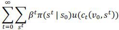
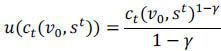
where we assume the power utility with risk-aversion coefficient γ:
There is no aggregate uncertainty. The only event that each household faces is a stochastic
idiosyncratic labor supply shocks. Each event si takes on values on a discrete grid S ≡ {s1, ⋯ , si, ⋯ , sl}. The idiosyncratic shock s follows a Markov process with a transition probability π(s'|s). We assume the law of large numbers holds so that the transition probabilities can
be interpreted as the fractions of agents making the transition from one state to
another. In addition, we assume that there is a unique invariant distribution  (s) in each state s. Again, by the law of large numbers (s) is the fraction of agents drawing s in every period. We denote st as the history of shock realizations:
st = (s0, s1, ⋯ , st−1, st)
We assume that an aggregate labor supply is perfectly inelastic for all periods and
denote it as  . An agent’s labor supply (hours worked) is denoted by
· s
We normalize the average idiosyncratic labor supply shock to be one.
1 = ∫ stdΦt
The output in the economy is produced using a single technology that exhibits constant returns to scale:
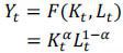
where F (· , · ) is a production function, and Kt and Lt denote the aggregate capital input and the aggregate labor input respectively. We use a Cobb-Douglas production function with capital income share α ∈ [0, 1].
The feasibility constraint for the economy is that the output can either be consumed or invested in the capital stock of the next period:
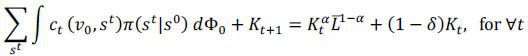
where δ ∈ [0, 1] denotes the depreciation rate of capital.
2. Enforcement Technology
Following Kehoe and Levine (1993) and Kocherlakota (1996), this literature commonly assumes that in the decentralized economy, households are excluded from financial markets forever when they default. We assume a more severe punishment upon default: households are not only excluded from the contingent claims markets forever but also (1) its current wealth is seized by the creditor and (2) it cannot receive any lump-sum transfer from the government. That is, the household loses all of its assets and income flows but its labor income cannot be garnished by the creditor. Hence, its only source of income beginning from the default period will be its labor income. The household who defaults at period t will have the following simple budget constraints for ∀τ ≥ t:
cτ = ωτsτL
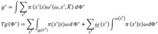
The autarky value Vaut at period t can therefore be written as:
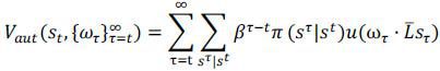
where ωt denotes the wage rate.
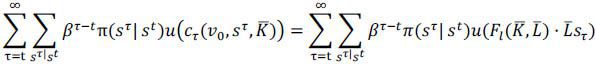
The households face an enforcement constraint. That is, the allocations are constrained so that planner makes them better off than autarky in every possible node in history:
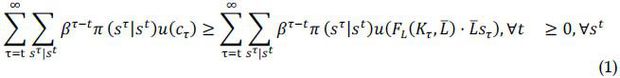
For the autarky value in the planner’s problem, we substitute the marginal product
of labor FL(Kτ, ) for the wage rate ωt from the equilibrium condition.
3. Planner’s Problem
As in Kochelakota (1996) and Alvarez and Jermann (2000, 2001), we set up the planner’s problem to discuss the constrained efficient allocations.
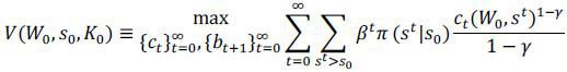
Planner is assumed to be benevolent so that he maximizes the social welfare:
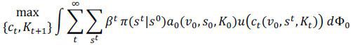
Subject to

where α0 is a Pareto weight assigned to the each agent by the planner and v0 is initial promised utility.
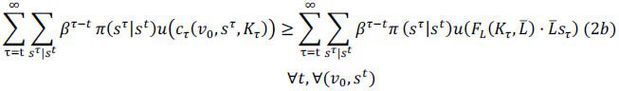
Planner maximizes the social welfare subject to constraints (2a) and (2b). Constraint (2a) is a feasibility constraint which must hold for all t and constraint (2b) is an enforcement constraint which must hold for all t and all (v0, st) and implies that each agent’s continuation value in the risk-sharing pool (i.e. each agent's continuation value of staying in the economy) should be at least as large as the value of autarky for all t and nodes. Let the Lagrangian multipliers on (2a) and (2b) be θt(Kt) and βtπ(st|s0)μt(v0, st,Kt) respectively.
In order to make the problem recursive, we can define cumulative multipliers: ξt(v0, ηt, Kt)3
,
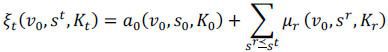
where sr is a subsequent history of st. We can rewrite cumulative multiplier recursively
ξt(v0, st, Kt) = ξt−1(v0,st−1, Kt-1) + μt(v0, st, Kt), ξ0(v0, s0, K0) = α0(v0, s0, Kt)
where {ξt(v0, st, Kt)} is a non-decreasing stochastic process.
The Lagrangian can now be written as
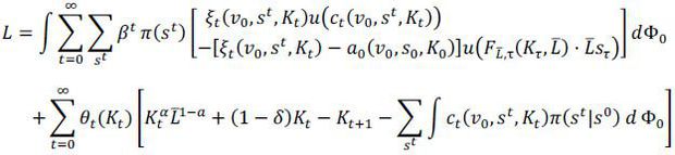
The next step is to derive the first-order necessary conditions. The first-order conditions are the following:

Equation (3) is the first-order condition with respect to an individual agent's consumption. θt is an aggregate variable since it is the shadow price of the feasibility condition. ξt is a summary statistic of an agent’s history. It measures how severely and how many times the agent has been constrained in his history. Therefore, equation (3) implies that the agent’s consumption is history-dependent and that the agent’s consumption should be higher if he has a higher ξt. We will characterize the agent’s consumption allocation in the next section.
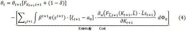
Equation (4) is the first-order condition with respect to aggregate capital investment Kt+1. The first line of the equation is a standard Euler equation. This Euler equation, however, contains the second term which we call the externality cost. This is the additional cost that the planner must pay in order to keep the agent from defaulting. This term contains (1) all the multipliers on enforcement constraints as summarized by the shadow prices (costs) of the enforcement constraints ξt − α0(= μ1 + ⋯ + μt+1), and (2) an increment in per-period autarky value when the capital stock is increased by one unit. To see how one unit of capital affects the externality cost term, consider the effect of such a change on capital stock at period T. This change will increase marginal product of labor, thereby increasing autarky values (that are solely dependent upon labor income) and making autarky more tempting. This change will affect all autarky values - and hence all enforcement constraints - prior to period T, and as a result increase the cumulative multiplier. We will also characterize the capital allocation in the next section.
4. Characterization of Constrained Efficient Allocations
In this section, we characterize the constrained efficient allocations. We will first characterize an agent’s consumption allocation and the shadow price of one unit of consumption next period. Second, we will discuss the capital allocation and externality cost that the planner encounters when he makes a capital investment decision.
1) Consumption Allocations
Enforcement constraints introduce a stochastic element into the consumption share of each household. The household’s initial promised utility, v0 determines its initial Pareto weight α0 and this weight governs the household’s consumption share in all future states of the world. When there are no enforcement constraints, the household’s consumption share is constant over time:
where 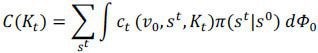 ,
,
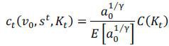
However, when enforcement constraints exist, the Pareto weights become stochastic and so does the household’s consumption share. The household’s consumption is characterized by the same linear risk sharing rule:
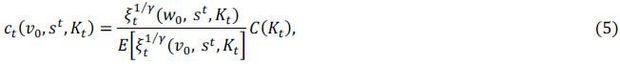
where 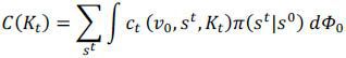
The household’s consumption share is stochastic. Recall that ξt(ω0, st, Kt) is the sum of all enforcement constraints in history st plus the initial Pareto weight, α0, and that these cumulative multipliers stay constant until the household switches to a state with a binding enforcement constraint. When this occurs, the multipliers increase so that the enforcement constraint is satisfied with equality.
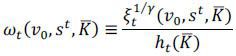
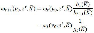
Let ht(Kt) denote the 1/γth cross sectional moment of the cumulative multiplier:
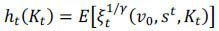
This process ht(Kt) is also a non-decreasing process and measures how many agents become constrained and how severely they are constrained.
This risk-sharing rule implies that when the household does not switch to a state with an enforcement constraint, its consumption share drifts downwards at the rate of the growth rate of ht(Kt). The derivation of the risk sharing rule is found in Lustig (2006).
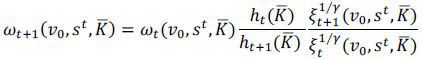
Next, we discuss the period t shadow price of one unit of consumption at t+1. Combining the risk sharing rules (5) and the first order condition (3) we obtain a expression for shadow price:
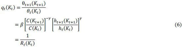
This shadow price contains the multiplicative adjustment cost of  . It measures the shadow cost of the enforcement constraints. As the growth rate of
h (Kt) in the economy increases, the cost of the enforcement constraints increases and
the more the planner needs to compensate at t+1. Hence the price of one unit of consumption increases.
. It measures the shadow cost of the enforcement constraints. As the growth rate of
h (Kt) in the economy increases, the cost of the enforcement constraints increases and
the more the planner needs to compensate at t+1. Hence the price of one unit of consumption increases.
2) Capital Allocations
In this part, let us characterize the capital allocation. We can rewrite equation (4) together with equations (3), (5) and (6) as follows:
1 = qt(Kt)[FK,t+1 + (1 − δ)] − Xt+1
Where
The above Euler equation would be a standard one if it did not contain the positive term Xt+1 on the right hand side. As a result of this extra term, the standard marginal return of investing one unit of capital exceeds the marginal cost of giving up one unit of consumption in constrained efficient allocations. Hence, there is an additional cost to the planner such that in equilibrium, the marginal benefit is equal to the marginal cost. We call the term Xt+1 the “externality cost of capital investment”. We argue that this externality cost of capital investment induces the need for a tax on capital income in order to make private agents internalize the externality in the decentralized economy.
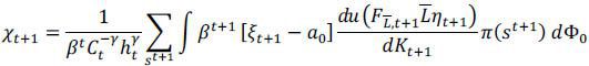
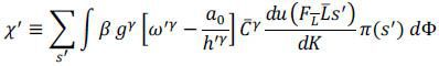
Externality Cost of Capital Investment Xt+1 : we now focus on the externality cost which is the last term on the right hand side of the Euler equation:
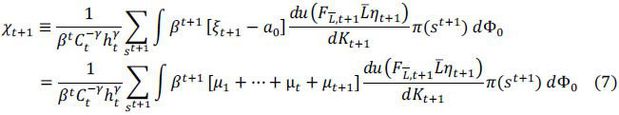
This externality cost of capital investment consists of three parts. First, there
is the incremental per-period autarky value 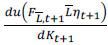 of a one unit increase of the capital stock. Second, the first part is multiplied
by the all the earlier multipliers as a shadow price (cost) of the enforcement constraints
[μ1 + μ2 + ⋯ + μt + μt+1]. Third, this externality cost of capital investment is normalized by the period
t price of consumption
of a one unit increase of the capital stock. Second, the first part is multiplied
by the all the earlier multipliers as a shadow price (cost) of the enforcement constraints
[μ1 + μ2 + ⋯ + μt + μt+1]. Third, this externality cost of capital investment is normalized by the period
t price of consumption  . Therefore, this is the cost at period t that the planner should pay if he wants to increase capital stock by one unit at
period t+1. In order for the planner to keep agents from defaulting, he needs to compensate
the agents more when he increases the capital stock.
. Therefore, this is the cost at period t that the planner should pay if he wants to increase capital stock by one unit at
period t+1. In order for the planner to keep agents from defaulting, he needs to compensate
the agents more when he increases the capital stock.
Proposition 2.1 Externality cost of capital investment Xt+1 is positive unless the full risk-sharing is feasible from initial period.
Proof. Proof is straight-forward from equation (7). Full risk-sharing means that no agent is constrained and this implies that μt(v0, st)= 0, ∀t and ∀(v0, st) by Khun-Tucker.
Proposition 2.2 Externality cost of capital investment Xt+1 is zero if the value of autarky does not depend on the capital investment.
Proof. Proof is straight-forward from equation (7). If 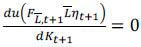 , then X should be zero.
Ⅲ. Characterization of Steady State Allocation
We open this section with a definition of the steady state. We define the steady state to be a state where all aggregate variables and the distribution of agents stay constant. We assume that the economy converges asymptotically to the steady state. It is important to note that even though the aggregate state will be stationary in steady state, each agent’s consumption will still fluctuate over time.
In this section, we also explain how we compute the steady state allocations. To summarize, consumption allocations and shadow prices are computed for a given capital level, K ; we then pin down the optimal steady state capital stock, given steady state individual consumptions, c(v0, st,K), shadow price R, and the invariant distribution, Φ.
1. Steady State Consumption Allocation
In this subsection, we discuss the individual household’s steady state consumption allocations. Throughout this subsection, we take the steady state capital stock K as given and then compute the steady state consumptions, a shadow price and an invariant distribution. In the next subsection, we will discuss how to decide the steady state capital stock K*.
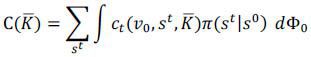
For a given capital stock K, the aggregate steady state consumption C(K) is:
C(K) = F(K, L) − δK
and we know this aggregate consumption should be allocated across the agents.
We use consumption weights as state variables instead of cumulative multipliers because we want stationary state variables. By (5), the consumption share of a household (v0, st,K) is defined as:
Notice that the individual’s consumption share is history dependent and its dynamics can be described as follows: when the agent (v0, st) does not switch to a state with a binding constraint, its consumption share next period drifts downwards to:
By (5), when the agent (v0, ηt) does switch to a state with a binding constraint, its consumption share in next period is
Proposition 3.1 (Lustig (2006)) When the agent (v0, st) switches to a state with a binding constraint, its consumption share equals to some cutoff level that does not depend on the history st; if the labor supply shock is first-order Markov.
Proof. When the agent is constrained, the participation constraint is satisfied with equality;
,
Now, if the labor supply shock s is first-order Markov, then the value of autarky in the right hand side of the enforcement
constraint does depends on the current realization of the shock st. This implies that  cannot depend on st, but on only st.
2. Determination of the Shadow Price
Proposition 3.2 For a given steady state capital stock K, if there is a unique invariant distribution Φ* with no aggregate uncertainty, then there is a stationary equilibrium in which shadow interest rate R* is unique and constant.
Proof. Again we follow Lustig (2004).4 If there is a unique Φ*, then it is clear that there is a unique growth rate:
and then this implies that there exists a unique constant shadow price R∗ that clear the markets.
3. Steady State Capital Allocation
The optimal capital K* is pinned down such that the steady state euler equation (8) is satisfied.

where
 is an individual agent’s consumption share tomorrow. This records how the degree
to which one agent has been constrained by the enforcement constraints over his history
since it contains all previous multipliers in it including the initial Pareto weight.
We subtract the initial consumption share since we do not have a enforcement constraint
at time 0. The initial consumption share part
is an individual agent’s consumption share tomorrow. This records how the degree
to which one agent has been constrained by the enforcement constraints over his history
since it contains all previous multipliers in it including the initial Pareto weight.
We subtract the initial consumption share since we do not have a enforcement constraint
at time 0. The initial consumption share part  will approach zero as time approaches infinity since h is a non-decreasing sequence. Then the aggregate steady state consumption to the
power of γ multiplied by an agent’s consumption share tomorrow to the power of γ is the inverse of the agent’s marginal utility of consumption at t+1. Finally, we convert the marginal utility of labor income with respect to capital
investment,
will approach zero as time approaches infinity since h is a non-decreasing sequence. Then the aggregate steady state consumption to the
power of γ multiplied by an agent’s consumption share tomorrow to the power of γ is the inverse of the agent’s marginal utility of consumption at t+1. Finally, we convert the marginal utility of labor income with respect to capital
investment,  , into time t+1 units of consumption by multiplying by
  .
.
Ⅳ. Decentralization with Solvency Constraints and Capital Income Taxes
Consider now decentralizing the constrained efficient allocations as a competitive equilibrium with capital taxes and solvency constraints. With these two instruments, the government can mimic the distorted first order conditions that define the constrained efficient allocations. The role of solvency constraints is the same here as in Alvarez and Jermann (2000; 2001). The role of capital taxes is to make the households internalize the externality cost that capital investment creates.
There are two assets available. We have a complete set of contingent claims bt+1(st+1; W0, ηt) at price qt. This is a security that pays one unit of consumption good at t+1 if st+1 is realized at t+1. The other asset is capital asset Kt+1, which yields the return of rt+1.
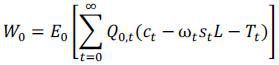
Instead of using the initial promised utility v0 to label the agents, we will use the initial wealth W0. So each household will be indexed by a pair of (W0, s0). We will show how to construct the initial wealth below.
Firms
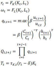
Firms operate production technology through a production function, F(Kt, Lt). At period 0, taking a sequence of pre-tax wage rates {ωt}, market interest rates {Rt}, and corporate profit taxes τK as given, a firm chooses a sequence of capital stocks Kt+1 and labor demand Lt that maximizes the discounted after-tax profit function:
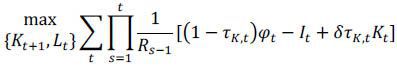
subject to
Where φt is corporate profit (capital income) and ῶt equals (1−τL,t)ωt. Note that it is firms that must pay the tax, which is imposed on income paid to physical capital.
The firms’ problem yields the following first order conditions:

where  is an intertemporal price. Based on these optimal conditions, firms make decisions
on labor demand and capital investment.
is an intertemporal price. Based on these optimal conditions, firms make decisions
on labor demand and capital investment.
Households
A household of type (W0, s0) chooses a sequence of consumption  and a sequence of contingent bonds
 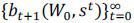 to maximize his expected lifetime utility:
subject to the usual budget constraint:
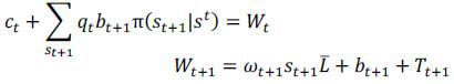
and a solvency constraint, one for each state:
bt+1(st+1; W0, st) ≥ Bt+1(st+1; W0, st),
given a sequence of prices and policies 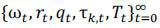
Government
The government collects tax revenue from financial intermediaries and transfers it to households in a lump-sum fashion such that her budget constraint is the following:
Tt = τk,t(rt − δ)Kt
Notice that we don’t have any government spending in this model.
1. Competitive Equilibrium
Definition 4.1 A competitive equilibrium with capital income tax {τkt} and solvency constraints{B t+1} for initial distribution Φ0 over (W0, s0) and capital stock K0 consists of a set of allocations, {ct(W0, st)},{bt(W0, st)}, and {Kt}, a set of prices, {rt}, {ωt} and {qt} and policies {τk,t, Tt} such that (1) Given the set of prices and policies, the allocations solve the household’s problem,(2) Given the set of prices, the allocations solve the firm’s problem, (3) the government budget constraint holds, (4) the resource constraints hold and (5) the markets clear;
Definition 4.2 Following Alvarez and Jermann (2000), borrowing constraints are not too tight if they Satisfy
V(Bt, st,Kt) = Vaut (st, Kt) ∀st
The link between enforcement constraints in the planner’s problem and solvency constraints in the household’s problem is the following. When an enforcement constraint in the planner’s problem binds, the corresponding solvency constraint in that state will bind. This condition guarantees that the borrowing constraints prevent default by not letting the agent accumulate more debt than they are willing to pay back.
Definition 4.3 The price of the contingent claims are not too high if the infinite sums of the form are finite for all equilibrium object xt+j
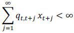
This condition guarantees that in a decentralized equilibrium, the present value of any allocation is finite. We use it to show that the value of the constructed assets is finite and that the household’s transversality condition holds.
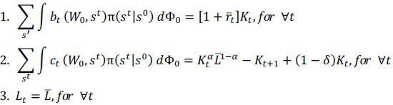
Proposition 4.1 Given allocations {ct(W0, st)} and {Kt} that satisfies
-
1. the feasibility condition at any period,
-
2. the enforcement constraints at any period and any state,
-
3. that the implied price of contingent claims are not too high and
-
4. that the marginal utility of consumption stays finite:
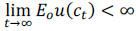
then there exist processes {bt(W0,st), Bt, rt, ωt, qt, Tt} such that sequences {ct(W0, st)}, {bt+1(W0, st)} and {Kt} compose a competitive equilibrium given the prices {rt, ωt, qt}, the solvency constraints {Bt+1} and the taxes on capital income {τk t}. In addition, the borrowing constraints are not too tight.
Proof. See the Appendix.
2. Steady State Capital Tax
This subsection explains how we compute the steady state capital tax rate. Equation (10) is the planner’s Euler equation, upon which the planner bases his capital investment decision and Equation (11) is the financial intermediaries’ no arbitrage condition in the competitive equilibrium. We choose the steady state tax rate such that these two equations are consistent with each other.


In order for the second welfare theorem to hold, two Euler equations should be equivalent and consistent and the capital tax rate can be backed out of the following equation:

Proposition 4.2 If X(K*) = 0, then  = 0.
= 0.
Proof. Proof is straight-forward from equation (12)
Ⅴ. Concluding Remark
We study optimal capital taxation under limited commitment. We prove that the optimal tax rate on capital income should be positive in steady state and should be increasing over time provided that full risk-sharing is not feasible.
A one unit increase of capital investment by an agent increases all individuals’ autarky values in the economy and generates externality costs in the economy. This externality cost provides a rationale for positive capital taxation even in the absence of government expenditure. Moreover, even with an aggregate uncertainty, this externality of capital investment still provides a theoretical role of positive capital taxation.5
In addition, a positive capital tax rate is induced by the existent of the capital investment externality, regardless of the size of aggregate uncertainty. The level of the tax rate however should be dependent on the current level of capital stock, as we can see equation (7) and (12).
To the best of our knowledge, this is the first paper to study optimal capital taxation in a limited commitment environment. Furthermore, this paper studies a model of risk-sharing to the fiscal policy literature and suggests that risk-sharing has important consequences in designing the optimal fiscal policy and should not be overlooked. For further study, one can quantitatively evaluates the optimal long-run capital tax rate.
Appendices
1. Invariant Probability Measure in Steady State
Given the monotonicity assumptions we must impose on π, we know that the consumption weight ω stays within a closed domain W because we know that ω ∈ [ω(s1,K), ω(sn, K)] since g is bounded. If some agent starts with an initial weight α0 ≥ ω(sn, K) his consumption weight drops below ω(sn,K) after a finite number of steps unless there is perfect risk sharing.
Let W = [ω(s1, K), ω(sn, K) and B(W), P(S) be the set of Borel sets of W and the power set of S respectively. The cutoff rule together with the transition function π for the labor shock process jointly defines a Markov transition function on shock realizations and consumption weight: Q: (W × S) × (B(W) × P(S)) → [0, 1] where

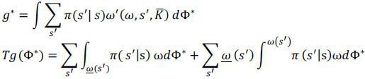
Given this transition function, we define an operator T∗ on the space of probability measures Λ((W × S), (B(W) × P(S))) as
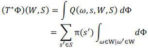
for all (W, S) ∈ B(W) × P(S). Note that T∗ maps Λ into itself.1 A fixed point of this operator is an invariant probability measure. Let Φ∗ denote the invariant measure over the space ((W × S), (B(W) × P(S))) that satisfies invariance:
T∗Φ∗(W, S) = Φ∗
In this section, we address the question of whether such a probability measure exists and is unique. Intuitively, this invariant measure describes the long-run cross- sectional distribution of the agent’s consumption shares implied by the planner’s social welfare maximizing policies.
Proposition 5.1 For a steady state capital stock K , there exists a unique invariant probability measure, Φ.
Proof.
This proof follows Lustig (2004) 2. We define an operator on the space of probability measures Λ((W × S), (B(W) × P(S))) as:
T*λ(W, S) = ∫ Q((ω, s), (W, S)) dλ
A fixed point of this operator is defined to be an invariant probability measure. To show there exists a unique fixed point of this operator, We check condition M in (Stokey, Lucas, and Prescott (1989), p.348). If this condition is satisfied, we can use Theorem 11:12 in Stokey, Lucas, and Prescott (1989) p.350. To be perfectly general, let W = [ω(s1, K), ωm ax]. There has to be an ε > 0 and an N ≥1 such that for all sets W, S
QN(ω, s), (W, S)) ≥ ϵ and QN((ω, s), (W, S)c) ≥ ϵ
It is sufficient to show that there exists an ϵ > 0 and an N ≥1 such that for all (ω, s) ∈ (W, S): QN((ω, s), (ωm ax, Sn)) ≥ ϵ, but we know that Q((ω, s), (ωm ax, Sn)) ≥ π(sn|s). If ωm ax ≥ ω(sn, K) then define

where N is finite unless there is perfect risk sharing. Then we know the QN((ω, η), (ωm ax, ηn)) ≥ ϵ where
ϵ = π(sn|s) · (π(sn|s))N−1.
If ωm ax ≤ ω(sn, K), the proof is immediate by setting ϵ = π(sn|s). This establishes the existence of a unique, cross-sectional distribution.
2. Proofs
Proof of Proposition 3.3
Again we follow Lustig (2004)3. If there is a unique Φ∗, then It is clear that there is a unique growth rate:
and then this implies that there exists a unique constant shadow price R∗ that clear the markets.
Proof of Proposition 4.1
By construction, first construct the equilibrium prices and transfer as follows
Next, construct the initial wealth and the asset holdings as follows:
and
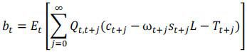
Under condition 4, these sums are well-defined. Finally, the construction of the solvency constraints (borrowing limits) is identical to that in Alvarez and Jermann (2000, 2001). If
qt,t+1· uc,t > βuc,t+1
then set Bt+1(ηt+1; W0, ηt) = bt+1 otherwise set Bt+1 = −Et[Qt,t+1(ωtηtL + Tt)]. For t > 0, the tax on capital income is backed out from the financial intermediaries’ no arbitrage condition
1 = qt,t+1[1 + (1 − τk,t+1)(rt+1 − δ)]
so that Rt+1 = 1 + (1 − τk,t+1) (rt+1 − δ) is set equal to 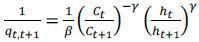 , for t = 0, we set R0 = 1. To check the constructed assets are budget feasible and that the transversality
conditions for the household are satisfied. We use the budget constraint to construct
asset holdings at each time and state so allocations are budget feasible. Budget constraints
together with government budget constraint and market clearing condition guarantee
that the allocations are also resource feasible. It is easy to show that the transversality
condition for the bond holds,
, for t = 0, we set R0 = 1. To check the constructed assets are budget feasible and that the transversality
conditions for the household are satisfied. We use the budget constraint to construct
asset holdings at each time and state so allocations are budget feasible. Budget constraints
together with government budget constraint and market clearing condition guarantee
that the allocations are also resource feasible. It is easy to show that the transversality
condition for the bond holds,

is satisfied assuming that
which is satisfied by condition 4.
Notes
Alvarez and Jermann (2000, 2001), Kehoe and Levine (1993), Kehoe and Perri (2002, 2004), Kocherlakota (1996), Krueger (1999), Lustig (2006) and among others. Moreover, Abraham and Carceles-Poveda (2007) study a similar economy and show a higher capital accumulation in the long run as a result.
In theirs, there are two countries (agents) and tax rates are different for each country (agent).
See also Atkeson and Lucas (1995). See also Krueger (1999): Lemma 16, 17, 19 and 21, and Theorem 18 and 21.
Capital accumulation dynamics with aggregate uncertainties is not discussed in this paper. With aggregate uncertainty, the distribution of agents becomes one of the key variables, which limits our further analysis.
See also Atkeson and Lucas (1995). See also Krueger (1999): Lemma 14, Corollary 14 and Theorem 15.
See also Atkeson and Lucas (1995). See also Krueger (1999): Lemma 16; 17; 19 and 21, and Theorem 18 and 21
References
(1995). Optimal Capital Income Taxation With Incomplete Markets, Borrowing Constraints, and Constant Discounting. Journal of Political Economy, 103, 1158-1175, https://doi.org/10.1086/601445.
, & (2006). Dynamic Optimal Taxation with Private Information. Review of Economic Studies, 73, 1-30, https://doi.org/10.1111/j.1467-937X.2006.00367.x.
, & (2001). Quantitative Asset Pricing Implications of Endogenous Solvency Constraints. Review of Financial Studies, 14, 1117-1152, https://doi.org/10.1093/rfs/14.4.1117.
, & (1992). On Efficient Distribution with Private Information. Review of Economic Studies, 59, 427-453, https://doi.org/10.2307/2297858.
, & (1995). Efficiency and Equality in a Simple Model of Unemployment Insurance. Journal of Economic Theory, 66, 64-85, https://doi.org/10.1006/jeth.1995.1032.
(1986). Optimal Taxation of Capital Income in General Equilibrium with Infinite Lives. Econometrica, 54, 607-622, https://doi.org/10.2307/1911310.
, & (1996). Asset Pricing with Heterogeneous Consumers. Journal of Political Economy, 104, 219-240, https://doi.org/10.1086/262023.
, , & (2003). Optimal Indirect and Capital Taxation. Review of Economic Studies, 70(3), 569-587, https://doi.org/10.1111/1467-937X.00256.
(1993). The Risk-free Rate In Heterogeneous-Agent Incompleteinsurance Economies. Journal of Economic Dynamics and Control, 17(5~6), 953-969, https://doi.org/10.1016/0165-1889(93)90024-M.
(1985). Redistributive Taxation in a Simple Perfect Foresight Model. Journal of Public Economics, 28, 59-83, https://doi.org/10.1016/0047-2727(85)90020-9.
, & (2002). International Business Cycles with Endogenous Incomplete Markets. Econometrica, 70, 907-928, https://doi.org/10.1111/1468-0262.00314.
, & (2004). Competitive Equilibria with Limited Enforcement. Journal of Economic Theory, 119(1), 184-206, https://doi.org/10.1016/S0022-0531(03)00255-2.
, & (2001). Liquidity Constrained Markets Versus Debt Constrained Markets. Econometrica, 69(3), 575-598, https://doi.org/10.1111/1468-0262.00206.
(1996). Implications of Efficient Risk Sharing without Commitment. Review of Economic Studies, 63, 595-610, https://doi.org/10.2307/2297795.
, & (1985). The Equity Premium: A Puzzle. Journal of Monetary Economics, 15, 145-165, https://doi.org/10.1016/0304-3932(85)90061-3.