
Borrowing Constraints and the Marginal Propensity to Consume
Abstract
Available evidence suggests that the average marginal propensity to consume (MPC) from the 2001 tax rebate in the US was not nearly as large as that from previous tax cuts. We examine if this phenomenon can be explained by the fact that the widespread use of credit cards has made borrowing accessible for most US households by constructing a model that simulates the dynamic effect of relaxed borrowing constraints. Our model uses Kreps-Porteus preferences which account for independent measures of relative risk aversion and the elasticity of intertemporal substitution, both of which can theoretically affect the willingness to save or spend. Our model shows that the average MPC drops substantially immediately after borrowing constraints are relaxed because few consumers have binding borrowing constraints at that time. The model also shows that consumers gradually reduce their wealth after borrowing constraints are relaxed, causing more of them to have binding constraints over time, which in turn causes the average MPC to rise gradually to a new steady state value that is slightly lower than the original value. This dynamic pattern of the MPC suggests that a greater ability to borrow with credit cards could explain the lower effectiveness of the 2001 tax rebate. In addition, the model predicts that consumers choose to hold lower amounts of liquid assets for precautionary reasons when they have a greater ability to borrow unsecured debt.
Keywords
Marginal Propensity to Consume, Borrowing Constraints, Precautionary Saving, Elasticity of Intertemporal Substitution, Tax Cut, 한계소비성향, 차입제약, 예비적 저축, 시점 간 대체탄력성, 조세 감축
JEL Code
D91, E21, E62, H31
Ⅰ. Introduction
To counteract the prolonged effects of the financial crises in several countries, many governments have tried to cut taxes and to raise their spending. G20 countries in 2009 agreed to stimulus packages worth an average 2% of GDP. The effectiveness of such fiscal stimulus policies depend on the marginal propensity to consume (MPC) from changes in income for the average consumer, but economists continue to debate the empirical value of the average MPC and the effectiveness of fiscal stimulus policies more generally. In particular, some empirical studies have argued that the MPC from income shocks has declined during the last one or two decades by estimating the MPC from the 2001 tax rebate and comparing it to that from previous tax-cuts. For example, Shapiro and Slemrod (1995) found that 43% of surveyed consumers were willing to spend the temporary increase in their take-home income in response to the changes in income tax withholding in 1992, even though the temporary increase in income was likely to be offset by a decrease in a tax refund or an increase in tax payments in 1993. Using a similar survey, Shapiro and Slemrod (2003) reported that only 22% of respondents were willing to spend the initial 2001 tax rebate in 2001. Although the authors use the same survey methodology and similar questionnaires, the differences in the responses are perplexing. 1
The differences in the survey responses indicate that the average MPC has changed. Furthermore, when we use assumptions about the distribution of the MPC across consumers in Shapiro and Slemrod (2002), we are able to calculate that the average MPC has fallen from approximately 0.47 in 1992 to approximately 0.33 in 2001.2
Other evidence is consistent with the hypothesis that the average MPC has declined over time. A University of Michigan survey, cited in the Christian Science Monitor, reported that only $8.36 billion out of the $38 billion 2001 tax rebate checks was spent. Also, a New York Times/CBS News poll in May 1982 found that approximately 50% of consumers in a survey said that they would spend the increase in take-home income due to the tax cuts proposed by the Reagan administration (Souleles (2002)), while Gallup Poll in July 2001 reported that only 17% of respondents said that they would spend the 2001 tax rebate (Shapiro and Slemrod (2002)).
Other empirical studies also indicate that the recent average MPC is no larger than the average MPC from two decades ago. Souleles (2002) estimates the average MPC in response to the 1982 tax cut to lie between 0.662 and 0.998 at a 5% significance level one year after the tax cut was implemented. Johnson, Parker, and Souleles (2006) estimate the average MPC in response to the 2001 tax cut to lie between 0.2 and 0.4 at a 10% significance level for the first three month period when the rebate was received. The authors then show that the estimated overall MPC rose to about 0.66 at a 10% significance level six months after the 2001 rebate was received, and that the MPC thereafter was small and insignificant.
Souleles (2002) and other authors have speculated that the apparent differences in the average MPC over time can be explained by a mental accounting hypothesis, where consumers save a large portion of a large lump-sum payment, but spend a large portion of incremental amounts from paychecks. (See Thaler (1990) for a general explanation of this hypothesis.) The foundation for this speculation is that the 1982 tax cuts and the 1992 withholding change were delivered to households through a reduction in taxes withheld from paychecks, while the 2001 tax cuts were delivered by mailing tax rebate checks.
However, we investigate a different explanation for the estimated fall in the average MPC out of temporary income shocks by using the fact that widespread use of credit cards has made borrowing accessible for most US households. The 2001 Survey of Consumer Finances (SCF) reports that 76.2% of the US households have at least one credit card and two thirds of households hold positive amounts of credit card debt (see Aizcorbe, Kennickell and Moore (2003) and Laibson, Repetto and Tobacman (2003)). In addition, credit card debt has grown over 10% per year since the 1970s, implying approximately a 250% growth rate per decade (see Yoo (1998)). Using results from Castronova and Hagstrom (2004) and the 2001 SCF, we show in Table 1 that the ratio between the median total credit limit from credit cards (as a measure of unsecured borrowing potential) per household and the median income per household has risen from approximately 0.3 in 1992 to nearly 0.5 in 1998 and 2001.3
To analyze the theoretical relationship between the average MPC and borrowing constraints, Carroll and Kimball (1996) compare a model with uncertainty and complete borrowing constraints to one where consumers have perfect foresight and can borrow as much as they like, as is typically assumed in the permanent/life-cycle income hypothesis. The authors show that the introduction of uncertainty and borrowing constraints causes the predicted average MPC to rise relative to the perfect foresight and unconstrained case and that the predicted MPC rises more for consumers with low amounts of liquid wealth than for those with high amounts of liquid wealth. Ludvigson (1999) shows that consumption responds to expected changes in consumer credit and suggests that increases in access to credit may induce less excess sensitivity of consumption to predictable changes in income. Using the constant relative risk aversion (CRRA) utility function, however, Carroll (2001) argues that a high growth rate in income and/or a high rate of discounting enjoyment in the future (or specifically the “impatience” of consumers) are the main factors that determine the MPC, rather than borrowing constraints per se. Kimball and Weil (2009) separate the effects of risk aversion and the willingness move resources across time and examine how these two effects determine precautionary saving in a two-period Kreps-Porteus model.
We extend Kimball and Weil‘s (2009) analysis by using a specific form of Kreps-Porteus preferences called Esptein-Zin preferences, which can be used in a multi-period simulation of how consumers may want to save or to borrow over time. More specifically, this paper also studies the theoretical effect of relaxing borrowing constraints on the average MPC, but it extends previous work in two directions. It uses the Kreps-Porteus preferences 4 in a multi-period model 5 instead of the commonly used CRRA preferences and analyzes the dynamics of the average MPC as well as its steady state predicted values.
Kreps-Porteus preferences are useful because they allow independent representations of risk aversion and intertemporal substitution, both of which may independently affect how much people want to spend and save. Relative risk aversion represents how much people dislike changes in the amount of resources they have over time due to external risks that they have no control over (such as a job loss caused by company wide layoffs). The elasticity of intertemporal substitution represents how willing people are to save and borrow over time (to substitute resources intertemporally) given a change in the relevant interest rate. Furthermore, as borrowing constraints are relaxed, our model shows that the willingness to save for precautionary reasons will decrease more when risk aversion is low, thereby raising the MPC from additional income available today. But as borrowing constraints are relaxed, willingness to borrow future resources may increase more when the elasticity of intertemporal substitution is high, thereby lowering the MPC from additional income available today. Thus, these two effects may offset each other under CRRA preferences due to the inverse relation between relative risk aversion and the elasticity of intertemporal substitution. With Kreps-Porteus preferences, however, we are able to control the size of these two effects independently by identifying separate parameters for the elasticity of intertemporal substitution and relative risk aversion. (See Kreps and Porteus (1978)).
We also consider how the average MPC from temporary income changes and the amount of assets may change over time until these values become stable in a self-defined steady state, where the mean, median and standard deviation of the distribution of cash-on-hand do not significantly change after many iterations (up to 100 periods). When borrowing constraints are relaxed in the model to simulate greater borrowing capacity through credit cards, the model predicts two effects. First, fewer consumers should have binding borrowing constraints at that time, so that more consumers would be able to smooth intertemporal consumption by saving or borrowing given preferences about intertemporal substitution. Also, after borrowing constraints are relaxed, consumers with a precautionary motive to save can afford to reduce the level of precautionary assets given preferences about risk aversion. Thus, we study the dynamics of the average MPC immediately after a change in borrowing conditions and thereafter as consumers adjust their precautionary wealth. We have found that the decline of the average MPC immediately after relaxing borrowing constraints is comparable to the estimated drop in the MPC, while the decline of the MPC at the new steady state can explain 10%-20% of the estimated drop. To the degree that borrowing constraints were relaxed in the US in early 2000s, our model can then partially explain empirical findings from previous studies.
The structure of this paper is as follows. Section 2 presents an optimization problem for a representative consumer with uncertain labor income and with a specified amount of credit card borrowing potential; it then explains how the analysis in this paper is conducted. Section 3 examines simulation results from the initial steady state before borrowing constraints are relaxed to the new steady state after they are relaxed, and then examines the path of the average MPC over time. Section 4 offers concluding remarks.
Ⅱ. The Model and Simulation Methodology
1. The Model
Rather than relying on behavioral assumptions, we examine whether a model with forward-looking consumers who respond optimally to changes in credit availability can explain the apparent decline in the average MPC out of temporary income shocks.
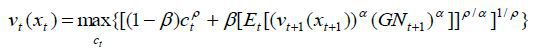
Formally, we model a representative consumer who is assumed to want to maximize the benefit from consumption resources over time according to the following specification of Kreps-Porteus preferences:

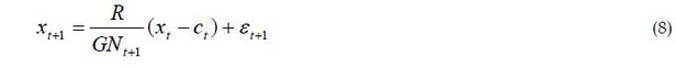
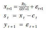
subject to:


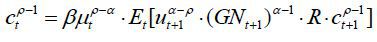
where Et denotes the conditional expectation given information at time t, β ∈ (0,1) is related to the future discount factor in the Epstein-Zin specification
of Kreps-Porteus preferences,6 R denotes the gross interest rate on a single, risk-free asset, Ct denotes a composite measure of consumption expenditure at time t, Yt denotes labor income at time t, and Xt denotes resources, or "cash-on-hand", available for consumption. Pt is the expected long run average or “permanent” component of income from labor services,
and εt and Nt are temporary and permanent changes in labor income, respectively. εt can be interpreted as temporary bonuses, lay-offs or illnesses without sick leave,
while Nt can be interpreted as promotions or demotions in one‘s career. G, the gross growth rate of Pt, is assumed to be constant and is meant to reflect the long run average growth rate
of the macroeconomy and real income. The logarithm of labor income shocks, ln εt and ln Nt, are assumed to be independently, identically, and normally distributed with mean
zero and variances  and
and  , respectively. This assumption implies that zero income shocks will not occur with
positive probability.
, respectively. This assumption implies that zero income shocks will not occur with
positive probability.
Equation (1) shows the time-inseparable Epstein-Zin (1989) specification of Kreps-Porteus preferences, which allows separate parameters for the elasticity of intertemporal substitution and relative risk aversion, both of which may affect the willingness to spend or save. As borrowing constraints are relaxed, the willingness to spend additional income may fall on average because fewer consumers are completely constrained from borrowing. This effect would lower the average MPC from additional income available today as borrowing constraints are relaxed because of a greater ability to borrow from future resources instead. Additional income available today could be saved or used to repay debt, another form of saving, instead of used to increase consumption expenditure. In addition, the relaxation of borrowing constraints weakens the precautionary saving motive, as Carroll and Kimball (2001) show with a CRRA model. Consumers should feel less of a need to maintain assets to protect against unforeseen income shocks when they are able to borrow in the event of unexpectedly low income. Predicted levels of assets therefore fall as borrowing constraints are relaxed as long as consumers are impatient, so that when the optimal consumption function is concave, the slope of the function—the MPC—will rise as wealth falls. The first effect, which we call the intertemporal substitution effect may be influenced by the elasticity of intertemporal substitution if its value affects the willingness to borrow, in particular at low levels of wealth when the ability to borrow is more likely constrained. The second effect, which we call the precautionary dissaving effect, increases when consumers have lower risk aversion, since precautionary saving—an example of prudence—is directly related to relative risk aversion.
In a CRRA model, these two effects may interfere with each other, since the elasticity of intertemporal substitution is constrained to be the inverse of relative risk aversion. However, even if these two effects offset each other, it is possible to obtain a clearer prediction of how these two effects change when the elasticity of intertemporal substitution and relative risk aversion independently change in a Kreps-Porteus model.
The parameter α is negatively related to relative risk aversion, which is equal to 1–α. The parameter ρ is directly related to the elasticity of intertemporal substitution, which is equal to 1/(1–ρ). The commonly used CRRA utility function is a special case of Kreps-Porteus preferences when α = ρ.
While equations (1) through (4) (and (6)) are conventional, equation (5) is different from previous models in that it allows the representative consumer to borrow up to a constant fraction of permanent labor income (kPt) , where k ≥ 0 and k is known to consumers. The model simplifies reality by assuming that k (as well as preferences, interest rates and the growth of real income from labor services) is exogenous and constant across time and across consumers, although to make the model more realistic we may want to allow k to depend on the endogenous level of permanent income, which does vary across time and across consumers. A change in the borrowing limits of credit cards or in consumer loan scores would change the borrowing capacity for consumers and is modeled as changes in k. When k = 0 , the representative consumer is not allowed to borrow at all, and as k increases, the borrowing constraint (5) is relaxed. Thus, borrowing constraints are modeled as quantity constraints rather than price constraints, i.e., rather than a gap between borrowing and lending rates. Consistent with this model, Jappelli (1990) presents evidence that consumers who are unable to borrow or “discouraged” from borrowing from financial institutions frequently are young (without an established credit history) and have low income, two characteristics that can proxy for permanent income.
Equation (6) says that the representative consumer must pay back all debts before he dies. In other words, he cannot declare bankruptcy during his lifetime after borrowing exogenous resources.
Maximization problems like the one above have no analytic solution due to uncertainty in future labor income, and thus require numerical analysis in order to obtain a solution. In the analysis, we take advantage of the recursive nature of the problem and then by normalizing all variables by Pt to reduce the number of state variables.7 After normalization, the constrained maximization problem (using a value function that represents the maximized utility function) is written as

subject to:


Lower-case variables represent upper-case variables normalized by the value of permanent income: xt+1 = Xt+1 / Pt+1 , xt = Xt / Pt and ct = Ct / Pt. The function vt represents the value function of resources today normalized by Pt , and the function vt+1 represents the value function of resources in the next period normalized by Pt+1.8 For a programming exercise, we set a finite time period T and also constrain the Kreps-Porteus problem to the terminal condition (10).
We solve the above problem under two sets of "impatience" parameter values, β = 1/1.05, R = 1.02, G = 1.02 and β = 0.9598, R = 1.0344, G = 1.03. The parameter values in the first set are from Ludvigson and Michaelides (2000) and those in the second set are either estimates in Gourinchas and Parker (2002) (in the case of β and R) or are the baseline values from Carroll (1997) (in the case of G). Based on empirical estimates from Carroll (1992), the standard deviations σε and σN are both set equal to 0.10. In the analysis, we use approximations of the distributions of εt and Nt by selecting a finite set of discrete points from the distributions.9
In order for the finite horizon results of the numerical analysis to converge to the infinite horizon solution, the “impatience condition” must hold. Epstein and Zin (1989) outline two impatience conditions for Kreps-Porteus preferences, depending on the elasticity of intertemporal substitution. When the elasticity of intertemporal substitution is greater than 1 (when ρ is greater than zero), the impatience condition equals

When the elasticity of intertemporal substitution is less than one (when ρ is less than zero), the impatience condition equals

where eis equals the elasticity of intertemporal substitution. We focus on (11b) in the Kreps-Porteus simulations because (11a) fails to hold for our specification of the interest rate and the growth rate of income. We do, however, use the case where the elasticity of intertemporal substitution equals one, a knife-edge case between (11a) and (11b).
Bishop (2008) derives a non-separable impatience condition that is independent of the value of the elasticity of intertemporal substitution when the growth rate of income is bounded:

where δ is a function of the elasticity of intertemporal substitution, relative risk aversion, exogenous variables that define the state of nature for consumers (the level of assets, the expected or average growth rate of income and changes in income), the benefit (utility) that we feel from consuming resources, the interest rate that we can earn from saving resources or the interest rate that we must pay when borrowing resources, and β, which represents how we feel about the trade-off between consuming resources today versus in the future.10 An interesting characteristic of δ is that it depends on the state of nature and it approaches zero when consumers are borrowing constrained, making (12) easy to satisfy for a finite interest rate. In simulation results provided below, we satisfy (11b) and (12) to be sure that the optimal consumption functions converge after several iterations.
The impatience conditions are labeled such because they are satisfied when consumers are impatient (i.e., β is low); but they can also be satisfied when the growth rate of income is high, making the future income look high relative to present income. Although the effect of the interest rate is ambiguous in (11b), when the return on saving is low in (11a), present consumption looks attractive relative to future consumption, and consumers become more impatient. Regardless of the underlying cause, when these conditions are satisfied and borrowing constraints are relaxed, the representative consumer is willing to borrow from future resources rather than save for the future.
2. Simulation Methodology
In the simulations, we focus on an increase in k from 0.3 to 0.5 to reflect the median total credit limit relative to the median income per household from 1992 to 2001, as shown in Table 1.11
<Table 1>
The Relaxation of Borrowing Constraints, 1992-2001
Notes: a The unit is 1998 US dollars. b The unit is 2001 US dollars. c The source is Castronova and Hagstrom (2004). d The source is the authors‘ calculation from 2001 SCF. e The source is Kennickell (2000). f The source is Aizcorbe et al. (2003). Bank type cards are credit cards issued by Visa, Mastercard, Discover and Optima.
We compute the optimal consumption functions for both values of k using backward induction, starting from a terminal period T = 100, sufficiently long to allow the consumption functions to converge according to the condition ct+1 – ct < 0.000001 for the highest level of normalized cash-on-hand, where t represents an arbitrary period.
Figure 1 represents changes in the optimal consumption function as borrowing constraints change under the second set of impatience parameter values.12 As k increases, the consumption function shifts up and to the left, implying less saving or greater borrowing to achieve a fixed level of consumption, or more intuitively, greater consumption at a fixed level of resources. This finding suggests that even consumers who are not currently constrained also increase spending as borrowing capacity increases, a claim consistent with Gross and Souleles (2002). Those authors find that consumers who are not currently borrowing constrained increase their consumption slightly in response to an increase in borrowing capacity from credit cards. They argue that consumers with non-binding constraints raise their consumption due to a weakened precautionary saving motive after borrowing constraints are relaxed.
We use these converged consumption functions, which approximate the optimal consumption function for an infinite horizon problem, to define the MPC out of temporary income shocks and evaluate its properties as the borrowing parameter k and the parameters governing the elasticity of intertemporal substitution and relative risk aversion change. We calculate the MPC for each consumer from the following equation:

Thus, equation (13) measures the MPC from “temporary” income changes, such as those from the tax code change in 1991 or the tax rebate in 2001. We calculate the average of (13) across consumers with different levels of cash-on-hand.
Using the optimal consumption function, we simulate the behavior of 4,000 consumers to examine the dynamic pattern of the MPC out of temporary income changes when the entire population experiences the same change in k but each individual experiences different simulated exogenous income changes. Income shocks are randomly drawn from log normal distributions based on empirical evidence from the Panel Study of Income Dynamics (See Carroll (1992)). To simplify the analysis, we assume that consumers do not start their working lives with any saved assets.13 Given this zero initial endowment and beliefs about expected future income, each consumer is programmed to optimally decide how much to consume and save each period over his lifetime. Given this behavior, the population of consumers generates a simulated distribution of normalized assets and normalized cash-on-hand that achieves a stable mean, median and standard deviation over time when the impatience conditions are satisfied.
After calculating the average MPC from the stable distribution of normalized cash-on-hand for k = 0.3, we increase k to 0.5, compute the corresponding optimal consumption function and then recalculate the average MPC from the distribution of normalized cash-on-hand during each period after the change in borrowing capacity until a new steady state is reached.
Ⅲ. Simulation Results
In this section, we present the dynamic pattern of the average MPC from the simulation to understand whether greater borrowing capacity could reduce the effectiveness of tax rebates in stimulating consumption expenditure.
Figures 2 and 3 plot the simulated average MPC out of temporary income changes over time. Time 0 indicates the initial steady state when the borrowing constraint parameter, k, is equal to 0.3, and Time 1 indicates the period during which the borrowing constrains are relaxed from k = 0.3 to k = 0.5. For comparison, the estimated MPC in the years of 1992 and 2001 are marked as two horizontal dotted lines. Under the assumptions about the distribution of the MPC across consumers in Shapiro and Slemrod (2002), the average MPC is estimated to have fallen from 0.47 in 1992 to 0.33 in 2001. When the risk aversion coefficient (rra) is one (two or three) and the elasticity of intertemporal substitution (eis) is one (1/2 or 1/3), the results in Figures 2 and 3 can be interpreted as those under ordinary CRRA preferences with the CRRA coefficient being one (two or three). Because we can put independent values for rra and eis, we can better predict the effects of changes in the average MPC with the Kreps-Porteus preferences.
Figures 2 and 3 show that when the borrowing constrains are relaxed from k = 0.3 to k = 0.5, the average MPC drops immediately and substantially because consumers have a weakened precautionary saving motive and therefore are predicted to reduce their assets. During this time, few consumers have binding borrowing constraints unless they suffer from an enormous negative income shock. As a result, additional temporary income from a tax rebate or tax cut is predicted to be mostly saved for future consumption so that the average MPC in the current period is predicted to be low.
However, consumers are predicted to reduce their assets in response to the loosening borrowing constraints when the impatience conditions are satisfied. As assets are spent, more consumers will face binding borrowing constraints even with greater borrowing capacity, so that the average MPC is predicted to rise gradually to a new stable value. Figure 4 shows the dynamic pattern of the fraction of the population with binding constraints, which corresponds to that of the average MPC: after falling substantially when borrowing constraints are relaxed, it subsequently rises gradually. The average cash-on-hand declines gradually as the weakened precautionary saving motive causes consumers to reduce their assets. Both a growing fraction of consumers who are borrowing constrained and lower cash-on-hand cause the average MPC to rise after its initial drop.14
Figures 2 and 3 also show that the magnitude of the initial decrease in the predicted average MPC from the simulation approximately equals the estimated decrease in the average MPC for some of the specified parameter values. For example, the magnitude of the decrease in the average MPC is slightly larger than the estimated decrease in the average MPC when rra = 1 and eis = 0.33 with the first set of impatience parameters.
[Figure 2]
Dynamic Pattern of the MPC during the Transition: R=1.02, G=1.02, β=1/1.05
Notes: Time 0 indicates the initial steady state with k = 0.3, while Time 1 indicates the period during which the borrowing constrains are relaxed from k = 0.3 to k = 0.5. The estimated MPC in the years of 1992 and 2001 are also marked as the two horizontal dotted lines. ‘eis’ denotes the elasticity of intertemporal substitution and ‘rra’ denotes the risk aversion coefficient in Kreps-Porteus preferences.
[Figure 3]
Dynamic Pattern of the MPC during the Transition: R=1.0344, G=1.03, β=0.9598
Notes: Time 0 indicates the initial steady state with k = 0.3, while Time 1 indicates the period during which the borrowing constrains are relaxed from k = 0.3 to k = 0.5. The estimated MPC in the years of 1992 and 2001 are also marked as the two horizontal dotted lines. ‘eis’ denotes the elasticity of intertemporal substitution and ‘rra’ denotes the risk aversion coefficient in Kreps-Porteus preferences.
After the initial drop, the average MPC gradually increases to a stable value, which we call a steady state value. Table 2 compares these steady state values when k = 0.3 and k = 0.5. Although the average MPCs in the steady state with k = 0.5 is lower than that with k = 0.3, the magnitude of the decline is much smaller than the estimated decline from the survey evidence. The magnitude of the decline in the average MPC at the steady state is between 0.013 and 0.030 depending on parameter values, which represents approximately 10% to 20% of the estimated decline. We conclude that as borrowing capacity increases the intertemporal substitution effect immediately lowers the average MPC from additional income available today, but this effect is substantially offset over time by the precautionary dissaving effect which raises the average MPC from additional income available today.
<Table 2>
Borrowing Constraints and the MPCs at the Steady State
Notes: Each column shows the average MPC across 4,000 consumers.
While the initial decrease in the MPC is comparable with the estimated decrease in the MPC (from 0.47 to 0.33), the decrease in the MPC between two steady states is much smaller. That is, when borrowing constraints are initially relaxed, the ability to borrow at the level of currently available resources reduces the willingness to spend additional income. But over time, liquid wealth is predicted to be reduced due to impatience and the precautionary dissaving effect, so that the willingness to spend additional income increases relative to the initial decrease.
In addition, Figure 4 shows that consumers will hold lower amounts of cash-on-hand when they have a greater ability to borrow unsecured debt due to the precautionary dissaving effect. This result is consistent with that of Bishop (2008).
[Figure 4]
Dynamic Pattern of the Binding Fraction and the Cash-on-Hand during the Transition
Notes:‘eis’ denotes the elasticity of intertemporal substitution and ‘rra’ denotes the risk aversion coefficient in Kreps-Porteus preferences.
Thus, to the degree that credit became easier to obtain in the early 2000s in the US through credit cards and other forms of unsecured credit, our model predicts that the MPC will initially decrease by a magnitude that is similar to the estimated decrease, although as consumers are predicted adjust their savings over time in the simulated model, the magnitude of the simulated decrease decreases to about 10%-20% of the estimated value from previous studies.
Ⅵ. Conclusion
This study examines whether a model with relaxed borrowing constraints can replicate the apparent decline in the average MPC in the US. We theoretically analyze the dynamics of the average MPC by using a model with Kreps-Porteus preferences, which accounts for independent measures of preferences about risk aversion and intertemporal substitution. If the widespread use of credit cards indicates that consumers are less borrowing constrained than they were a generation ago, they should be better able to maintain a steady level of consumption expenditure over time (which we call the intertemporal substitution effect) and should have less incentive to save (which we call the precautionary dissaving effect). The model shows that the first effect is dominant immediately after borrowing constraints are relaxed and that the first effect is offset by the second effect gradually as consumers reduce their assets. The model likewise predicts that consumers are substantially less responsive to changes in income immediately after they acquire a greater borrowing capacity, although this effect diminishes over time as they reduce their assets. The results of this paper therefore suggest that temporary tax cuts or tax rebates will be less effective in boosting consumption expenditure when consumers have a greater borrowing capacity.
In addition to credit card borrowing, other types of household borrowing capacity may have also grown during the past few decades. Securitization and decreasing interest rates may have given consumers a greater ability and incentive to use home-secured debt for greater consumption expenditure (See Aizcorbe, Kennickell, and Moore (2003)). Future work could enhance the model in this paper by including durable goods or illiquid assets that allow consumers to borrow more secured debt.
Appendices
Appendix 1.
See Shapiro and Slemrod (2002) for the parameterization of the distribution of individual MPCs. m denotes the average MPC. To maintain non-negative a, c must be equal to or greater than 0.9850.
Appendix 2. How to Solve the Dynamic Optimization Problem under Kreps-Porteus Preferences
1. Reducing the Number of State Variables in the Maximization Problem
The value function is multiplicatively separable with respect to expected long run average income, so it can be normalized by this value to reduce the number of state variables from two to one. In effect, randomness in nature for consumers is reduced from two dimensions to one dimension, and consumers are modeled to have a lifetime perspective and care only about available resources relative to their expected long run average income, rather than available resources and expected long run average income separately.
Consider the value function in the second to the last period:
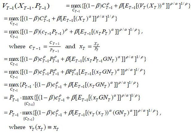
Consider  . For the second to the last period, VT–1 (XT–1, PT–1) = PT–1 · vT–1(xT–1). Using this solution, we can find VT–2(XT–2, PT–2) = PT–2 · vT–2(xT–2), and so on. In general, Vt (pXt, pPt) = pVt(Xt, Pt), where p = 1 / Pt ; that is, Vt(·) is homogenous.
Since the terminal period was chosen arbitrarily, we can find the solution to the
original problem in each period if we solve the normalized one-state problem vt(xt). That is,  implies
  for any t.
The problem for a representative consumer whose preferences are represented by the Epstein-Zin function therefore becomes
subject to:
where the lower case variables represent upper case variables normalized by Pt. Necessary conditions for maximization
To derive the first order condition of this normalized problem, assume that we have already found the optimal value function, v(x), for all periods except for t and t + 1. Perturb the allocation of resources in t and t + 1 such that the derivative of unmaximized normalized utility (ut) with respect to the choice variable is equal to zero:
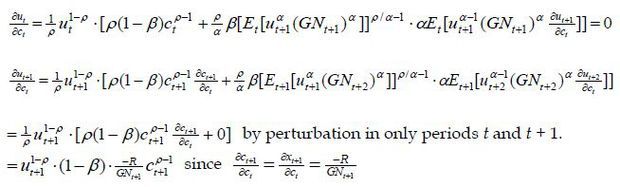
so that

which implies that

Let 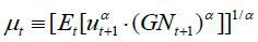 so that the first order condition is rewritten as
Note that  and the stochastic
  have inverse powers and if α = ρ, the first order condition results in the expected
utility first order condition. Note also that under certainty (when risk is irrelevant),
the expected utility first order condition results and the value function is a transformation
of the expected utility function.
have inverse powers and if α = ρ, the first order condition results in the expected
utility first order condition. Note also that under certainty (when risk is irrelevant),
the expected utility first order condition results and the value function is a transformation
of the expected utility function.
2. Backward Induction in the Maximization Problem
In the last period of life, it is optimal to consume all resources if there is no bequest motive. (If there is a bequest motive, then one could specify that it is optimal to leave a fixed amount at the end of life.) Since the future value function is modeled to be zero after death, the value function in the last period is defined as vT(xT) = xT. Given this extra constraint, we can iteratively solve for the optimal level of consumption expenditure in each period. Beginning with period T – 1, we specify a level of the normalized state variable and find consumption as a function of xT–1 from the first order condition:

If the representative consumer is not borrowing constrained, the first order condition
holds exactly. If he is constrained, we set cT – 1 = xT – 1 + k. To find the optimal level of consumption,  , we plug each solution to the above equation to find the one that maximizes

However, because the marginal utility of consumption and the marginal utility of saving are convex over the entire domain, there is a unique solution to the first order condition ∀t . After finding this unique optimal level of consumption expenditure in T – 1, we use the value vT – 1(xT – 1) to solve the first order condition in period T – 2. Thus, we proceed iteratively until we reach the beginning of the representative consumer's working life.
3. Discretizing the Distribution of Error Terms in the Maximization Problem
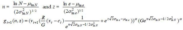
To approximate the integrals in the expected value operator, we construct a discrete approximation based on a one dimensional Gauss-Hermite quadature given that ln Nt+1 and ln εt+1 are normally distributed and independent. We use 10 discrete points from a one dimensional quadature for both ln Nt+1 and ln εt+1. Because multidimensional quadatures are extremely difficult to calculate, non-independent errors would be difficult to approximate. Expectations are modeled to be a function of probabilities of changes in the normalized state variable, conditional on information available today. From the independent normal distributions of ln Nt+1 and ln εt+1, we select 10 Gauss-Hermite discrete points from each distribution and weight them accordingly. (See Secrest and Stroud (1966) for the points and weights for a one dimensional Guass-Hermite quadrature.) The approximation of expected value (utility) of random cash on hand using this procedure is based on the following:
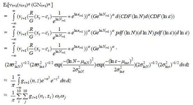
where CDF( ) is the cumulative distribution function of ( ), pdf( ) is the probability distribution function of ( ), and d represents the total derivative.
ωi is the weight for the ith discrete point of the distribution of n and ωj is the weight for the jth discrete point of the distribution of z for i, j = {1,2,…,10} such that 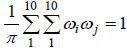 .
.
Thus, we can approximate the first order condition as:
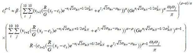
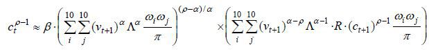
To make this equation easier to read, drop the arguments of the functions and let
 . The approximate first order condition reduces to
Let ct (xt) be the solution to this equation (and the approximate solution to the first order condition). The value function can be solved, given a level of liquid wealth xt for each solution ct (xt) and given that the problem has be solved for period t+1.

Notes
We are grateful to two anonymous referees for valuable comments, and also thank Aditya Goenka, Cheolsung Park and Eko Riyanto for helpful discussions. Cheolbeom Park acknowledges financial support from College of Political Science and Economics, Korea University. Any remaining errors are ours. The corresponding author is Cheolbeom Park.
Survey questions in Shapiro and Slemrod (1995) and Shapiro and Slemrod (2003) differ slightly: Shapiro and Slemrod (1995) asked whether the recipient would spend the temporary increase in take-home income, whereas Shapiro and Slemrod (2003) asked whether the tax cut would increase spending or saving. We can think of no reason of how the large difference in the survey responses can be explained by the subtle differences in the survey questions.
These calculations produce estimates that are fairly robust across different assumptions about the parameters used to specify the distribution of the MPC from Shapiro and Slemrod (2002). See the Appendix for perturbations of the average MPC when these distribution parameters change.
Ludvigson (1999) also shows that the ratio of consumer loans to personal income has also grown by more than 200% since World War II.
Epstein-Zin preferences are a mathematical specification of the more general Kreps-Porteus theory. We use Epstein-Zin preferences in our simulations, but refer to the preferences as Kreps-Porteus preferences in the paper where appropriate because of their generality and because the theory was created before the Epstein-Zin specification.
Haliassos and Michaelides (2000) also use Kreps-Porteus preferences in a multi-period model but focus on presenting computational techniques to solve household portfolio choice problems.
Bishop (2008) shows that in general the future discount factor in the Epstein-Zin specification depends on the state of nature (the level of available resources) and factors that influence the state of nature such as the growth rate of income, unforeseen changes in income, as well as the elasticity of intertemporal substitution, relative risk aversion and a measure (β) that represents how we feel about the trade-off between consuming resources today or consuming them in the future.
The state of nature for the representative consumer before normalization is described by the levels of permanent income and "cash-on-hand" or available resources to spend on current consumption.
The variables GNt+1, representing the change in permanent income each period, appears in the future value function vt+1 because the equation is normalized by current permanent income. Also, see Bishop (2008) for the steps involved in normalizing this function.
All analyses in this paper are done by Mathematica 5, and the programs are available upon request. Appendix 2 describes the optimization and simulation methods.

 where St is the value of saved assets.
The dynamic pattern of the MPC is robust for other values of k. The complete results when k = 0, 0.1, 0.2, 0.3, 0.5, and 0.6 are available upon request.
The shape and response of the optimal consumption function are qualitatively the same under the other set of impatience parameters.
We also used initial wealth estimates from Gourinchas and Parker (2002), but they had no substantial effects on the average MPC after several periods.
Figure 4 shows the dynamic pattern of the binding fraction and the cash-on-hand for eis = 0.5 under the first set of impatient parameter values and for eis = 0.33 under the second set of impatient parameter values. The plots under other combinations of eis and impatient parameter values are not reported to save space but they are qualitatively identical and available upon request.
References
, & . (2004). Risks for the Long Run: A Potential Resolution of Asset Pricing Puzzles. Journal of Finance, 59, 1481-1509, https://doi.org/10.1111/j.1540-6261.2004.00670.x.
(2001). A Theory of the Consumption Function, With and Without Liquidity Constraint. Journal of Economic Perspectives, 15, 23-45, https://doi.org/10.1257/jep.15.3.23.
, & (1996). On the Concavity of the Consumption Function. Econometrica, 64, 981-992, https://doi.org/10.2307/2171853.
, & . (2004). The Demand for Credit Cards: Evidence from the Survey of Consumer Finances. Economic Inquiry, 42, 304-318, https://doi.org/10.1093/ei/cbh062.
, & (1989). Substitution, Risk Aversion, and the Temporal Behavior of Consumption and Asset Returns: a Theoretical Framework. Econometrica, 57(4), 937-969, https://doi.org/10.2307/1913778.
, & (2002). Consumption over the Life Cycle. Econometrica, 70, 47-89, https://doi.org/10.1111/1468-0262.00269.
. (1990). Who is Credit Constrained in the US Economy? Quarterly Journal of Economics, 105, 219-234, https://doi.org/10.2307/2937826.
, , & (2006). Household Expenditure and the Income Tax Rebates of 2001. American Economic Review, 96(5), 1589-1610, https://doi.org/10.1257/aer.96.5.1589.
, & . (2009). Precautionary Saving and Consumption Smoothing across Time and Possibilities. Journal of Money, Credit and Banking, 41(2~3), 245-284, https://doi.org/10.1111/j.1538-4616.2009.00205.x.
, & (1978). Temporal Resolution of Uncertainty and Dynamic Choice Theory. Econometrica, 46(1), 185-200, https://doi.org/10.2307/1913656.
. (1999). Consumption and Credit: A Model of Time-Varying Liquidity Constraints. Review of Economics and Statistics, 81, 434-447, https://doi.org/10.1162/003465399558364.
, & . (2003). Consumer Response to Tax Rebates. American Economic Review, 93, 381-396, https://doi.org/10.1257/000282803321455368.
(2002). Consumer Response to the Reagan Tax Cuts. Journal of Public Economics, 85, 99-120, https://doi.org/10.1016/S0047-2727(01)00113-X.