I. Introduction

Countiries involved in trade disputes usually choose demand-side trade policy tools. Specifically, when there is a trade dispute or a trade ‘war’ between two countries, both countries choose trade policy tools that will exert negative demand shocks on the opposing country’s exports. Typical examples are tariffs and import quotas, both of which aim to reduce imports of the opposing country’s products.

Some trade disputes enter an entirely different phase. Occasionally, for example, exports of products which are indispensable intermediate inputs in the opposing country’s key sectors are directly regulated or even embargoed. A striking instance took place in August of 2020, when the United States announced new sanctions which prohibit any foreign company from supplying semiconductors produced using US technology to the Chinese company Huawei. In fact, the trade dispute between China and United States is said to have begun in 2018 or even years earlier, witnessing the use of many traditional trade policy tools, but recent policy tools would be regarded as supply-side tools in the sense that they affect the supply side of the market.

Japan’s decision strictly to control the export of three materials which are essential to the production of semiconductors and display panels in July of 2019 was another striking example of a supply-side trade policy. This policy, which was said to initiate the Korea-Japan trade dispute, triggered a fierce conflict between the two nations afterwards. Japan’s decision remains in place as of December of 2020.

Supply-side trade policy tools can be regarded as ‘strong’ or ‘extreme’ tools compared to demand-side tools, and trade disputes during which supply-side tools are employed tend to involve a greater variety of, and fiercer, phases. Usually, supply-side trade policy tools are not regarded as ‘traditional’ trade policy tools. Moreover, these tools affect the supply side of the controlled products directly, meaning that their impacts on both parties differ from the effects of demand-side tools. Additionally, the target country of supply-side tools, even when unspecified, is usually more obvious.

The purpose of this paper is to measure the impact of the Korea-Japan trade dispute on the Korean economy by means of a supply-driven input-output (IO) analysis. It is possible to apply a traditional demand-driven IO analysis mechanically by ‘pretending’ that the change in production was caused by a final demand shock. However, a demand-driven IO analysis can be used only when the shock affects the final demand and thus cannot be applied to the current situation. Supply-driven IO analyses have been used in various situations but have not been applied to trade disputes with supply-side trade policy tools.

The paper is organized as follows. Section 2 explains the motivation of the paper in more detail and reviews the literature. Sections 3 and 4 explain the methodology and the data, respectively, and the results of the paper are given in Section 5. Section 6 concludes the paper.

II. Motivation and Literature

Most trade disputes have significant impacts on the countries involved. Also, it is likely for trade disputes to escalate due to the involved countries’ efforts to have a greater impact on the opposing country so as to ‘win’ the dispute, causing the dispute to grow into a trade ‘war.’

Trade disputes can have various phases depending on many factors, such as the trade pattern between the countries involved, diplomatic relationships, political situations, the history of the disputes, and emotional factors, among others. The involved countries choose tools which may allow them to apply the strongest pressure on the opposing country. For example, demand-side tools such as tariffs or import quotas can be highly effective when the country is the biggest importer of the product in question.

Some policy tools affect the supply side of the products in question, as witnessed in the US-China and Korea-Japan disputes. In fact, the most influential and well-known incident of the use of a supply-side trade policy tool took place during the ‘first oil crisis’ in 1973-1974, when the Organization of the Petroleum Exporting Countries (OPEC) reduced the production of crude oil radically and began controlling oil exports strictly, though this was not a trade ‘dispute.’ A similar process was repeated in the ‘second oil crisis’ of 1979-1980; the world economy experienced skyrocketing oil prices and significant damage in almost every sector during and after these two crises.

The impact of demand-side policy tools on the opposing country can be measured using a standard demand-driven IO analysis, i.e., using the well-known formula (I - A^d)^-1 Δy , where I is the identity matrix, A^d is the domestic input coefficient matrix and Δy denotes the change in the final demand vector. This method, however, cannot be used for supply-side trade policy tools. Suppose that country A is the monopolistic producer of material AA, that AA is an indispensable raw material used to produce BB, and that BB is an important product in country B. Suppose that country A suddenly decreases their exports of AA. Unless country B succeeds in securing a substitute input for AA, the only option is to reduce the production of BB. Interrelated sectors will also be affected severely.

This type of impact cannot be computed using the above formula because the shock occurs on the supply side and because the formula above can be applied only to demand shocks. In a demand-driven IO analysis, the amounts of gross output and intermediate inputs are key endogenous variables, and they are determined by the final demand for the products, the major exogenous variables.

We have two options in this situation. The first is to apply the standard demand-driven IO analysis. While we are not supposed to apply a demand-driven IO analysis, we can still use this method, just as we can apply, e.g., the ordinary least square method when its assumptions are violated. We compute or assume a change in production due to the dispute and then assume that it was caused by a demand shock.

The second option is to use a supply-driven IO analysis. This was initially suggested by Ghosh (1958) and has been used in situations with supply-side shocks. However, the standard supply-driven IO analysis can be used only when the shock affects the value-added components, for example, a change in labor supply which affects the compensation of employees.

It is necessary briefly to explain the mechanics of a demand-driven IO analysis at this point. Upon the realization of a demand shock, the response of the supply side is to change production by the same amount because in IO analysis, the supply side is assumed to be infinitely elastic. This requires additional domestic intermediate inputs, imported intermediate inputs and primary production factors, of which the first is met by increases in production in the corresponding sectors, the second by imports, and the third by households. This is the second round, and the subsequent rounds are repeated infinitely in the same manner. The total impact is the sum of the impacts in each round, and we can compute the changes in production, value-added, imports and employment in individual sectors and in the entire economy as the sums of infinite geometric series. Considering that the analysis is interested in the sectors in the upstream which provide raw materials to the affected sector, we can refer to the impact of the shock in a demand-driven analysis as the ‘backward linkage effect.’

A supply-driven IO analysis is interested in the impact of the shock on the sectors downstream to which the affected sector supplies intermediate input. Suppose that the production of a sector is decreased as the result of a supply shock. The product of the affected sector is used as a raw material in other sectors, which implies that other sectors also experience a decreased supply of this raw material and will be forced to decrease their production. This chain reaction will proceed infinitely in the same manner. The total impact is the sum of the infinitely many impacts in each round, and we can compute the decreases in gross output, value-added, imports and employment in individual sectors and in the entire economy. Considering that the analysis is interested in the sectors downstream to which the affected sector supplies raw materials, we refer to this impact as the ‘forward linkage effect.’

In order to apply a supply-driven IO analysis, however, we need to modify the method slightly because the shock did not affect value-added but gross output. For this purpose, we ‘exogenize’ the ‘affected’ sector, the sector BB in the aforementioned example, that is, the sector in which the embargoed product is used as an essential input. If the supply of product AA, whether domestic or imported, is reduced and cannot be replaced, then the affected sector is forced to reduce its gross output. Therefore, the gross output of the affected sector can no longer be treated as an endogenous variable. The gross output of the exogenized sector is treated as an exogenous variable in the supply-driven IO analysis.

The first step in this method is to estimate the decrease in the production of the affected sector. It is important to note that at the outset of the dispute, the decrease in the production of the affected sector will depend on the decrease in the material in question but will be gradually relieved for several reasons, such as import substitution, diversification of suppliers, and/or an improvement of the dispute due to negotiations.

The analysis proceeds in two directions from this stage. The estimated decrease in the production of the affected sector is used to compute its backward linkage effect, i.e., its impact on other endogenous sectors and on the entire economy using an ordinary demand-driven IO analysis. In the opposite direction, its forward linkage effect is computed by means of a supply-driven IO analysis. The overall impact is the sum of the two effects.

The body of literature on the demand-driven IO analysis is enormous such that reviewing the literature is almost impossible. In fact, it can be said that the demanddriven analysis was the primary objective of Leontief’s invention of IO tables and his analyses. Reyes and Mendoza (2013) noted that out of two main identities inside the IO tables, “Leontief concentrated his attention on the first one (the one which leads to the demand-driven IO analysis, specifically the Leontief inverse matrix).”

The impact of most shocks which affect the final demand of an economy or can be converted into such shocks can be computed by means of a demand-driven analysis. Most government expenditures, changes in household consumption levels, firms’ new investment projects, and changes in exports are typical examples. In recent decades, many countries compute the economic impacts of public infrastructure projects using a demand-driven IO analysis to enhance the efficiency of public finance. Korea’s Prefeasibility Studies performed by the Ministry of Economy and Finance and the Korea Development Institute which began in 1999 represents a good example.

The demand-driven IO analysis has also been used to measure the impact of trade disputes. Tian and Yang (2014) conducted a demand-driven IO analysis to measure the impact of the EU-China trade dispute around photovoltaic products. They used China’s IO tables and computed the impact of antidumping on China’s export of photovoltaic products and on the GDP of China. An IO analysis was also applied to a political dispute. Wu et al. (2016) used a demand-driven IO analysis to measure indirect economic losses in China caused by the dispute over the Diaoyu Islands, or Senkaku Islands, in 2012, which affected China’s international trade.

The recent US-China trade dispute which started in 2017 invited a large number of studies. Considering the positions of the two countries in the world economy, the potential impact of the dispute, when it develops into a full-scale trade war, can be disastrous to most of their trade partner countries, not to mention themselves. For this reason, the dispute worried not only governments but also researchers all around the world, and almost every possible methodology has been employed to forecast the impact of the dispute.

Tyers and Zhou (2019) used a multi-region general equilibrium model and considered various scenarios to forecast the impact of the US-China dispute. Song and Lee (2018) used a computable general equilibrium (CGE) model to predict the economic impact of the US-China trade dispute. They considered several scenarios and forecasted the impacts on various macroeconomic variables of Korea as well as other countries involved.

Gentile et al. (2020) also applied a CGE model and used the Asian Development Bank’s Multiregional Input-Output Tables (ADB MRIOT) to measure the impact of the US-China trade dispute on the involved countries and on the world economy. Two scenarios were considered in their study: the current state as of May of 2019 (the first scenario) and a ‘full-scale tariff war’ (an additional 25% tariff on all imported products). They computed the impacts on various aggregate variables of the US, China and many trade partner countries, at the same time showing, however, that some countries would benefit from the dispute by absorbing some import demand from both countries.

Additionally, the demand-driven IO analysis was used in many studies to forecast the impact of the US-China trade dispute. We can think of two main reasons. First, the IO analysis is relatively easy to use, apply and adjust, and the computation is fast. It involves relatively simple matrix operations, which can be executed on most desktop computers. Second, more countries are producing IO tables in recent years, and in particular, the recent availability of multi-country IO tables such as the World Input-Output Database (WIOD) has made it easy to compute the impact of a demand shock on the countries included in the database.

Jung (2017) assumed that the trade dispute will reduce both countries’ mutual trade by 10% and computed the impact on the GDPs of China, the US, and Korea using a demand-driven analysis with WIOD. He estimated that Korea’s GDP will decrease by 0.35%, with the proviso that the estimate depends on numerous unexpected factors. Kim and Kim (2018) also used a demand-driven IO analysis and the WIOT to forecast the impact of the US-China trade dispute on the Korean economy. They estimated the impacts on various aggregate variables and provided policy recommendations for Korea.

Abiad et al. (2018) also utilized the ADB MRIOT to forecast the impact of the US-China trade dispute. The ADB MRIOT consists of the IO tables of 62 countries and 35 sectors, and in their study it was used to measure the impact on the GDP, exports and employment of developing ADB member countries as well as the US and developed European countries. They considered three scenarios: the status quo, ‘the worse’ scenario and ‘the worst’ scenario, also conducting a demand-driven IO analysis.

Xia et al. (2019) applied a demand-driven IO analysis to the 2013 edition of WIOD and forecasted the impact of the 2017 US-China trade dispute. The primary field of interest in their study was the energy sector, and they computed the impacts of the dispute in various scenarios on the GDP and energy consumption of not only the countries involved but also many of their trade partner countries.

Finally, a demand-driven IO analysis was also applied to the Korea-Japan trade dispute. Jeong et al. (2019) used the ADB MRIOT and computed the economic impact of the dispute on Southeast Asian countries using an indirect approach. They computed the contribution of Korea’s export of electronic components, including semiconductors, to the GDPs of these countries, from which they concluded that the decrease in Korea’s production of semiconductors due to the dispute could be detrimental to the Southeast Asian countries.

Jung et al. (2019) conducted the empirical study most pertinent to the motivation of this paper. They provided (i) the details and the expected consequences of Japan’s export control of the three materials in July of 2019, (ii) the history of Japan’s export of the three materials since their strengthening of export control and (iii) a reckoning of the aftermath of the dispute to Korea and Japan. For quantitative forecasts, they made two separate assumptions: (1) Korea’s production of semiconductors will decrease by 10%; and (2) Japan’s exports of chemical products, electronic equipment and machinery will decrease by 5%. Then they used a CGE model to predict the impacts on the Korean economy. They estimated that when Korea’s semiconductor production decreases by 10%, Korea’s GDP and total exports will decrease by 0.320~0.384% and 0.347~0.579%, respectively, depending on the monopolistic power of Korea’s semiconductor supply. They also predicted that Korea’s GDP and exports will decrease by 0.06% and 0.089%, respectively, as the result of the second assumption.

The supply-driven input-output analysis was devised by Ghosh (1958). He considered an economy in which firms’ behaviors differ from those in Leontief’s system. Clearly, both Leontief and Ghosh used the same input-output system, but Leontief assumed that the final demand is exogenous, the supply side is infinitely elastic, and the input coefficients are fixed or highly stable, whereas Ghosh assumed that value-added is exogenous and the distribution structure of the final products in terms of the composition of customers is fixed or highly stable. Two sets of assumptions, even with same tables, lead to two entirely different ways of analyzing the impacts of ‘shocks’ on endogenous variables, correspondingly referred to here as demand-driven and supply-driven IO analyses. Reyes and Mendoza (2013) compared the two types of analysis and provided a compact theoretical explanation of the difference and the relationship between them.

As described earlier, a supply-driven IO analysis can be applied when the production of a certain sector is affected due to an exogenous reason, in other words, when the gross output of a sector ‘must’ be reduced due to a reason unrelated to the final demand. While there can be a wide variety of causes, they can be sorted into three categories: (i) an exogenous shortage of labor such as a labor shortage due to a labor market mismatch and or a strike; (ii) an exogenous shortage of capital, that is, damage to the production capacity due to a natural disaster such as an earthquake or a flood, or non-natural causes such as accidents or a failed loan extension; and (iii) an exogenous shortage of intermediate inputs, especially when they cannot be easily replaced, caused by a natural disaster, e.g., a supply shortage of electricity due to an earthquake, or a non-natural accident, such as a reduction or stoppage of the supply of key materials, parts or components essential in a certain sector. Obviously, Japan’s decision strictly to control the exports of the three materials essential for producing electronic displays and semiconductors is one of the most pertinent examples of the third category.

Davis and Salkin (1984) measured the impact of an exogenous decrease in the supply of water to the agricultural sector of the Kern County, California, US, on the value-added of various sectors and the aggregate economy of the county using both ordinary demand- and supply-driven IO analyses. The impact on the county’s aggregate value-added computed from the supply-driven analysis was approximately 71% of that computed from the demand-driven analysis, and they concluded that the forward-linkage effect of the agricultural sector is weaker than the backward-linkage effect.

Chen and Rose (1986) studied the ‘joint stability’ of input and output coefficients theoretically and provided a short empirical work. As explained earlier, the demand-driven and the supply-driven IO analyses assume that input and output coefficients are fixed or highly stable, respectively. After the work of Ghosh (1958), many researchers studied if both sets of coefficients can be stable at the same time, in particular when the disturbance is not small. They showed that joint stability is theoretically possible, and provided an empirical example. They assumed that the supply of aluminum into Taiwan decreases by 50%, a major disturbance, assumed that output coefficients are fixed, and showed that the resulting changes in input coefficients are small at less than 1% in most sectors.

Groenewold et al. (1987) applied a supply-driven IO analysis to answer frequently asked questions in industrial and regional economics related to the ‘contribution of a certain industry to the total employment in a region.’ They addressed this issue by treating the industry in question as exogenous and applying a supply-driven IO analysis.

Roberts (1994) measured the economic impact of the quota on milk production on the UK economy using a modified IO analysis. She suggested that both backward and forward linkage effects be considered and showed that in the milk industry, the former type is more significant than the latter. Leung and Pooley (2002) estimated the economic impact of a 100% reduction in longline fishing on Hawaii’s economy. They claimed that a demand-driven approach is not appropriate because the shock was not initiated by the demand side, and they applied a supply-driven IO analysis to estimate the impact. Fernández-Macho et al. (2008) used a supply-driven IO analysis to estimate the impact of the reduction in the total allowable catch of cod and hake on the economy of Galicia, Spain. Seung and Waters (2009) also used a supply-driven approach to estimate the backward and forward linkage effects of the fishery sector in Alaska. They classified the fishery sector into multiple subsectors and measured their backward and forward effects separately. They also conducted numerous policy simulations and estimated various economic impacts.

Kim (2015) applied a supply-driven IO analysis to the case of the 2010-2011 outbreak of foot-and-mouth (FAM) disease in Korea, one of the most serious incidents of FAM in the world. He computed the backward and forward linkage effects of the outbreak on individual sectors and on the national economy, and identified the sectors with the strongest backward and forward effects. He also showed that the estimated impact by a supply-driven analysis is greater than that by a demand-driven analysis.

Studies in this field agree that a supply-driven IO analysis is desired when the exogenous shock affects production, not the final demand, because the standard demand-driven IO analysis does not capture all economic impacts. Obviously, Japan’s decision strictly to control the exports of three materials would directly affect production in the semiconductor and display sectors in Korea and not the final demands, which justifies the use of a supply-driven IO analysis. While the event fits the framework and satisfies the assumptions of the supply-driven IO type of analysis, empirical applications to the Korea-Japan trade dispute could not be found, and it is the goal of this paper to estimate the economic impacts in this manner. This paper follows the methodology adopted by Leung and Pooley (2002), Fernández-Macho et al. (2008), Seung and Waters (2009) and Kim (2015), all of which are based on Ghosh (1958).

III. Methodology

Let A^d be the n × n domestic input coefficient matrix of an economy, where n is the number of products/sectors. Also, let x and y^d be the n × 1 vectors of the gross output and domestic final demand, respectively. The market clearing conditions for domestic products can be expressed as x = A^d x + y^d , where the terms on the right-hand side represent the intermediate and final demand for domestic products, respectively. The solution to the market clearing condition is x = (1 - A^d)^-1y^d , or, equivalently,

The n × n matrix (I - A^d)^-1 is called the Leontief inverse matrix, and it measures the backward linkage effects. The (i, j) th element of (I - A^d)^-1 measures the change in the gross output of the i th sector when the domestic final demand for the j th product changes by one unit. Thus, the j th column of (I - A^d)^-1 gives the impacts of the domestic final demand for the j th product on the gross output of individual sectors.

Suppose an exogenous shock affects the gross outputs of particular sectors, and let n₁ be the number of affected sectors. Assume, without a loss of generality, that the affected sectors are the first n₁ sectors. As mentioned in the previous section, we can mechanically apply a demand-driven IO analysis, that is, we can apply (1). This implies we assume, incorrectly, that the exogenous shock affected the final demands of the n₁ sectors and that the magnitude of the shock is identical to the reductions in the gross outputs. In this case, the impacts of the shock on individual industries are represented by the first n₁ columns of (I - A^d)^-1 , that is an n × n₁ matrix.

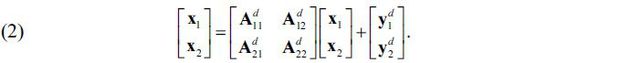
We now move to the supply-driven IO analysis, and we will derive the procedure for the backward linkage effect first. Let n₂ be the number of unaffected sectors; i.e., n₂ = n - n₁ . The market clearing condition for domestic products, x = A^dx + y^d , can be partitioned into the affected and the unaffected sectors, as follows:

Because the shock affects the first n₁ sectors, their gross outputs are not determined by their final demands. Accordingly, they are no longer endogenous. Hence, the first equation in (2) does not hold, and we only consider the second; i.e., 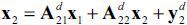. This is the market clearing condition for the n₂ unaffected sectors in which the x₂ variables are endogenous variables which depend on the exogenous variables x₁ and . We solve the equation for x₂ , and we get , or, equivalently,

assuming that . The n₂ × n₁ matrix measures the backward linkage effects of Δx₁ on x₂ .

Let B^d be the domestic output coefficient matrix; that is, . Here, is the share of the i th product out of the total gross output, which is used as the intermediate input in the j th sector. It can be interpreted as the direct forward linkage effect of the i th product on the j th sector, and is referred to as the ‘output coefficient,’ compared to the ‘input coefficient’ . Output coefficients are also called ‘allocation,’ ‘supply’ or ‘sales’ coefficients.

The decomposition of the total cost can be expressed as x' = w^d + w^m + v , where the left-hand side refers to total cost or total input while the terms on the right-hand side refer to the domestic intermediate input, the imported intermediate input and the value-added. We can show that w^d = x'B^d , and the above equation becomes

Upon solving (4) for x , we get x' = (w^m + v)(I - B^d)^-1 , or equivalently,

assuming that Δw^m = 0 . This result can be found in Ghosh (1958, p.61), Miller and Blair (2009, p.547), and in the Bank of Korea (2014, p.138). This formula gives the increases in the gross outputs of individual sectors when the value-added vector changes by Δv . The matrix (I - B^d)^-1 is called the ‘output inverse matrix’ or the ‘Ghosh inverse matrix,’ and it plays a role similar to that played by (I - A^d)^-1 in the demand-driven IO analysis.

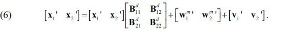
Equation (4) can be partitioned for the affected and unaffected sectors, as follows:

Because the shock affects the first n₁ sectors, the first equation in (6) does not hold, and we only consider the second, . In this equation, the x₂ variables are endogenous variables which depend on the exogenous variables x₁ and v₂ . We solve the equation for x₂ , and we get , or equivalently,

assuming that . The n₂ × n₁ matrix measures the forward linkage effects of Δx₁ on x₂ .

We have one more effect of the exogenous shock, which is the direct impact of the shock on x₁ , i.e., Δx₁ . It is the initial component of the shock from which backward and forward linkage effects proceed in the opposite directions, but it needs to be counted only once. In this paper, we will simply regard it as a component of the backward linkage effect. For this reason, we will stack an identity matrix of size n₁ × n₁ on top of and a zero matrix of size n₁ × n₁ on top of for the sake of notational and computational convenience.

In sum, we have three n × n₁ matrices of multipliers which measure the impacts of Δx₁ on x₂ ; (i) impacts computed using a standard demand-driven IO analysis given by the first n₁ columns of (I - A^d)^-1 , (ii) direct and backward linkage effects from a supply-driven IO analysis computed by , and (iii) forward linkage effects computed by . After these effects on gross outputs are computed, the impacts on value-added and employment can be computed by multiplying the value-added and employment coefficients.

IV. Data

As mentioned in section 1, we will apply the above method to the Korea-Japan trade dispute to measure its impact on the Korean economy. For this purpose, we used the IO tables of Korea in 2018, the most recent IO tables of Korea. Korea’s 2018 IO tables are available at four levels of sector classification, with 33, 83, 165 and 381 sectors, of which the tables with 83 sectors were used in this paper because they are the tables with the smallest number of sectors in which the semiconductor and electronic display sectors are separately represented.

In this paper, the 83-sector classification was rearranged into a 24-sector classification, in which the semiconductor and electronic display sectors were located in the beginning of the classification, as shown in Table 1.1 Gross output, value-added, exports and employment of these 24 sectors in 2018 are given in Table 2. Note that in 2018, the affected sectors, 1 and 2, account for approximately 5% of the total gross output and value-added in Korea, whereas they account for more than 20% of total exports.

TABLE 1

24-SECTOR CLASSIFICATION

TABLE 2

GROSS OUTPUT, VALUE-ADDED, EXPORTS AND EMPLOYMENT OF 24 SECTORS IN 2018

Source: Bank of Korea.

V. Results

In July of 2019, Japan announced the decision to tighten the export control of three materials: fluorinated polyimide, photoresist and hydrogen fluoride. Fluorinated polyimide is an essential material in the manufacturing of LCD and OLED display panels, which, in turn, are essential parts in the manufacturing of smartphones and televisions, which account for a major portion of the Korean economy. Photoresist and hydrogen fluoride are essential materials in the manufacturing of memory semiconductors, which not only constitute a substantial portion of the Korean economy but also are essential parts in the manufacturing of various ICT products and electronic equipment.

Table 3 confirms that Japan’s shares are substantial in Korea’s import of these three materials as well as in the world markets, while Korea’s shares in Japan’s exports are much smaller. Furthermore, the affected sectors represent a major portion of the Korean economy, and three additional sectors, in this case other electronic components; computer and peripheral equipment; and telecommunication, video, and audio equipment, would be severely affected because semiconductors and display panels are indispensable in these sectors. These five sectors accounted for 26.4% of Korea’s total exports, 6.7~6.8% of the total gross output and GDP, and 1.2% of total employment in 2018. See Table 4.

TABLE 3

MARKET SITUATIONS OF THE THREE MATERIALS

Source: KITA, July 1, 3 and 10, 2019.

TABLE 4

AFFECTED SECTORS IN THE KOREAN ECONOMY IN 2018

Source: Bank of Korea.

In order to apply the supply-driven IO analysis, we need to estimate, or at least make a rigorous assumption of, the magnitude of the direct impact of the shock on the gross output of the affected sectors, i.e., Δx₁ in equations (3) and (7). In other words, we need to estimate the changes in the production levels of the affected sectors.

This estimation is straightforward in some situations. In the work by Kim (2015), for example, the official numbers of culled animals infected by foot-and-mouth disease were published, from which the production decreases in the corresponding sectors could be estimated almost exactly. There are other situations in which a precise estimation of the change in production in the affected sector is straightforward. Production quotas are a typical example.

Unfortunately, however, this is complicated in some situations, specifically when the relationship between the shock and the direct impact is uncertain, as in the case of Japan’s export control. If the three materials are perfectly irreplaceable and if Japan enforces the embargo strictly, the production levels of Korea’s semiconductor and display sectors will then decrease by 91.9% and 93.7%, representing Japan’s shares in Korea’s imports of fluorinated polyimide and photoresist, respectively (Table 3).

However, these figures highly overestimate the actual impact even if the above assumptions are true because it is possible for the firms in these sectors to have accumulated sufficient inventories of the materials and prepare alternative materials while the stockpiles last. In this sense, the above figures could be regarded as the maximum level of the direct impact.

Hong (2020) computed the actual imports of the three materials before and after the shock using trade statistics, which are given in Table 5. That study found that (i) the import of fluorinated polyimide from Japan rather increased and that Japan’s share did not change much after the control, suggesting that Japan did not enforce the decision strictly. In addition, a Korean company succeeded in localizing the material. It was also found that (ii) the import of photoresist from Japan dropped significantly directly after Japan’s decision, but it recovered quickly to the level before the shock. Japan’s share decreased by 6.1%p from 92.8% to 86.7%, but was replaced by a detour import through Belgium. This was possible because Japan did not restrict the export of the material to Korea through a third country. In other words, the import of photoresist from Japan did not change much. Finally, it was found that (iii) the import of hydrogen fluoride from Japan dropped severely after Japan’s decision. A major portion of the import of this product was replaced by supplies from domestic firms and from Chinese and Taiwanese firms.

It can be concluded from Table 5 that the impact of Japan’s export control on production in the semiconductor and display sectors was insignificant. In fact, Hong (2020) concluded that the impact was limited. This conclusion, however, underestimates the impact on production in the affected sectors for many reasons. First, the data in Table 5 consider only the short-term impact and may underestimate the impact if the production levels of the affected sectors were increasing. Second, the data in Table 5 do not take the inventory of the materials into consideration and may underestimate the impact if the inventory levels of the materials were exhausted. Third, Japan’s decision has not changed since the outset of the export control, and it is possible that Japan will enforce the decision more strictly.

TABLE 5

IMPORTS OF THE THREE MATERIALS SINCE JAPAN’S EXPORT CONTROL

Note: Japan’s shares in this table are slightly different from those in Table 3.

Source: Hong (2020).

In order to estimate the direct impact more rigorously, the actual production and the exports of the affected sectors were also studied. First, the manufacturing production index of the semiconductor sector since 2017 is presented in Figure 1.2 Note that the production levels of semiconductors since July of 2019 were all larger than those in July of 2019. This can be regarded as an evidence that Japan’s decision did not have an impact on semiconductor production in Korea. However, the fluctuation in early 2020 may have stemmed from the unstable supply of the raw material, and the growth trend since early 2020 could be seen as slightly lower compared to the trend in 2019.

FIGURE 1.

MANUFACTURING PRODUCTION INDEX: SEMICONDUCTOR

Source: Statistics Korea.

Exports of semiconductors and displays and their year-on-year growth rates are given in Figures 2 and 3, respectively. As shown in Figure 2, exports of semiconductors and displays in 2019 were lower than those in 2018, resulting in negative growth rates in 2019, as can be observed in Figure 3. As shown in Figure 3, however, the growth rates of the exports of the two products (thick solid and broken curves) were lower than that of total exports (thin solid curve), even after the base effect was exhausted. Moreover, the gap is roughly 10%. If we interpret the total exports as an indicator of the global economic trend, the gap can then be regarded as an impact that cannot be explained by economic trends worldwide. It is possible that Japan’s decision was one of the causes despite the fact that it is not easy to determine the source of the gap quantitatively due to the insufficient number of observations.

FIGURE 2.

MONTHLY EXPORTS OF SEMICONDUCTORS AND DISPLAYS (AMOUNTS)

Source: Korea International Trade Association.

FIGURE 3.

MONTHLY EXPORTS OF SEMICONDUCTORS AND DISPLAYS (GROWTH RATES)

Source: Korea International Trade Association.

Considering the above information, we assume that the direct impact of Japan’s export control on the affected sectors is a 10% decrease in production; that is, the gross outputs of the semiconductor and display sectors decrease by 10% each as a result of Japan’s export control. Subsequently, we compute its impact on other sectors and on the national economy using standard demand-driven and supply-driven IO analyses. Thus far, Jung et al. (2019) present the only quantitative study of this issue, also assuming that Korea’s semiconductor production will decrease by 10%.

It should be noted that an IO analysis is linear and additive and that the results can therefore be used for various scenarios. When the production of the affected sectors decreases by 15%, for example, the impact on other sectors and on the national economy can easily be obtained simply by multiplying the results obtained later in this paper by 1.5.

Backward and forward linkage coefficients are given in Table 6. As mentioned earlier, the direct impacts of the shock, a 2×2 identity matrix, are included in the backward linkage effect coefficient vectors. According to Table 6, the overall backward linkage coefficients for semiconductors and displays were 1.2426 and 1.4505, respectively. This implies that the corresponding backward impacts of one-unit exogenous shocks in these two sectors on the upstream sectors which provide raw materials to these sectors are 0.2426 and 0.4505 units.

Table 6 shows that the business service sector is most severely affected by the shocks in both the semiconductor and display sectors, signifying that both sectors heavily depend on high-tech professional services. Chemical products, other electric and electronic products, and the utility, wholesale and trade and transportation sectors also receive significant backward linkage impacts from the shocks in the semiconductor and display sectors.

TABLE 6

BACKWARD AND FORWARD LINKAGE COEFFICIENTS ON GROSS OUTPUT ACCORDING TO THE SUPPLY-DRIVEN IO ANALYSIS

Source: Author’s computations.

The overall forward linkage coefficients were estimated at 0.0551 and 0.3420, respectively, implying that the forward impacts of one-unit exogenous shocks in these two sectors on the downstream sectors which use semiconductors and displays as raw materials are 0.0551 and 0.3420 units, respectively. Small forward linkage coefficients of semiconductors are rooted in the peculiar output structure in this case. Out of a total production amount of about 134 trillion won, only 7.4%, or close to 10 trillion won, is used as raw materials in the country, while most of the production, 123 trillion won, is exported. The share of intermediate demand as a percent of gross output is 36.5% for displays, and this share is greater for other manufactured products. Kim (2015) reports that the overall forward linkage coefficients for dairy cattle, beef cattle and swine are 1.318, 1.554 and 1.787, respectively, which are much greater than those for semiconductor and display panels.

The sector of other electric and electronic products is most severely affected by the shocks in both sectors, which is intuitive given that semiconductors and display panels are essential components in those sectors. The results of this paper also imply that machinery, transport equipment and construction are other important downstream sectors.

The first two columns of Table 7 are the sum of the backward and forward linkage coefficients, that is, the total coefficients from the supply-driven IO analysis, including direct impacts. The total supply-driven coefficients are 1.2977 and 1.7925. Table 7 also gives the demand-driven coefficients. This result shows that both sets of coefficients are very similar to each other. However, this result is not general, instead being a coincidence. In the work of Kim (2015), the supply-driven coefficients of the above-mentioned products (3.247, 3.724 and 4.110) were significantly higher than the demand-driven coefficients (1.942, 2.174 and 2.319).

The impacts of Japan’s export control scheme as represented by the reduction in gross output are computed in Table 8. This is obtained by multiplying the direct impacts, 13.4 and 6.4 trillion won, by the coefficients in Table 7. The total impact is estimated to be 29.0 trillion won, of which the contributions of the shocks in semiconductor and display sectors are 17.4 (60.2%) and 11.5 (39.8%) trillion won, respectively. The total impact consists of the direct impact (19.9 trillion won, 68.6%), the backward linkage effect (6.2 trillion won, 21.2%) and the forward linkage effect (2.9 trillion won, 10.2%). Electric and electronic products and the business services sectors are the sectors most severely damaged by the dispute.

TABLE 7

COEFFICIENTS OF GROSS OUTPUT FROM SUPPLY-DRIVEN AND DEMAND-DRIVEN ANALYSES

Source: Author’s computations.

TABLE 8

IMPACTS OF THE TRADE DISPUTE ON GROSS OUTPUT ACCORDING TO THE SUPPLY-DRIVEN INPUT-OUTPUT ANALYSIS

Source: Author’s computations.

The impacts of Japan’s export control on Korea’s GDP are given in Table 9. The total impact is estimated to be 13.6 trillion won. This consists of the contributions of the shock to the semiconductor sector (9.3 trillion won, 68.9%) and to the display sector (4.2 trillion won, 31.1%). The total impact consists of the direct impact (10.2 trillion won, 75.1%), the backward linkage effect (2.3 trillion won, 17.3%) and the forward linkage effect (1.0 trillion won, 7.6%). Electric and electronic products and business services sectors are the sectors most severely damaged by the dispute, also in terms of GDP.

TABLE 9

IMPACTS OF THE TRADE DISPUTE ON VALUE-ADDED ACCORDING TO A SUPPLY-DRIVEN INPUT-OUTPUT ANALYSIS

Source: Author’s computations.

Employment effects were also computed. The total reduction in employment was estimated to be 53,659 persons, with the contributions of the shocks on the semiconductor and display sectors being 27,290 (50.9%) and 26,369 (49.1%) persons, respectively. The total impact consists of the direct impact (14, 494 persons, 27.0%), the backward linkage effect (28,202 persons, 52.6%) and the forward linkage effect (10,964 persons, 20.4%). The patterns of the impacts on employment differ considerably from those on the gross output and value-added due to the difference in the average labor productivity levels among the sectors.

We can compare our results with those of Jung et al. (2019). We observed that the impacts of the Korea-Japan trade dispute as computed by demand-driven and supply-driven IO analyses are nearly identical and that when the gross output of the semiconductor sector decreases by 10%, Korea’s GDP is expected to decrease by 9.3~9.4 trillion won, which is 0.5% of the aggregate GDP. This is 30~67% higher than the estimate by Jung et al. (0.320~0.384%).

Not only it is difficult to trace the cause of the difference rigorously, but we cannot directly compare the accuracy or forecasting power of these results. There are two conceivable causes of the difference, however. First, an IO analysis, unlike other methodologies, takes the inter-relationships among sectors into account explicitly. Hence, an underestimation of the impacts is likely if inter-industry relationships are not considered. Second, on the other hand, the results of an IO analysis can be interpreted as ‘instantaneous’ magnitudes of the sectors’ responses to shocks. Accordingly, this method tends to overestimate the impact. This is similar to the slope of the tangent line of a concave increasing function, as an IO analysis assumes a Leontief production function, i.e., fixed proportions among production factors, but in reality, adjustments in firms’ behaviors take place such that the effects of shocks are mitigated over time.

VI. Conclusion

In this paper, we estimated the impact of the Korea-Japan trade dispute using a supply-driven input-output analysis. The Korea-Japan trade dispute, unlike typical trade conflicts which proceed into intensifying trade policy tools to affect the opposing country’s exports, began with Japan’s export control of three materials which are indispensable for the production of semiconductors and display panels, two key products in the Korean economy recently. Japan’s action, when effective, would inevitably result in a large-scale cutback in production in Korea and thus in severe damage to Korea’s GDP. Unlike typical trade conflicts, again, the shock is the supply-side version because the decrease in production was caused by a decrease in the supply of an intermediate input, which, in turn, was caused by an exogenous non-economic factor.

This makes the standard demand-driven IO analysis invalid, and a supply-driven IO analysis was adopted in this paper in order to estimate the impact of the Korea-Japan trade dispute. The supply-driven IO analysis was initially devised by Ghosh (1958) and later modified to incorporate supply-side shocks on gross output.

The results of this paper show that when the gross outputs of the semiconductor and display panel sectors decrease by 10% each, Korea’s aggregate gross output will decrease by 0.67% (29.0 trillion won), the aggregate GDP will decrease by 0.72% (13.6 trillion won) and employment will decrease by 0.22% (53,659 persons). When the gross output of only the semiconductor sector decreases by 10%, the decrease in the aggregate GDP was estimated to be 0.50% (9.3~9.4 trillion won). This is 30~67% higher than the estimate by Jung et al. (0.320~0.384%).

The results of this paper can be utilized in several ways. The method used in this paper is easy to apply and does not require complicated modelling compared to macro-econometric models or computable general equilibrium models. In addition, the results are linear and additive and can therefore be used in various scenarios.

The methods used in this paper can be extended to a multi-country setting. For example, we can measure the impacts of a supply-side shock caused by the Korea-Japan trade dispute not only on Korea but also on Korea’s major trade partners. The World Input-Output Database or the OECD’s Inter-Country Input-Output tables can be used for this purpose.

The result of this paper has many limitations. First, the direct impact of an exogenous shock, the crucial component of a supply-driven IO analysis, could not be estimated rigorously. We ‘assumed’ that the gross outputs of the semiconductor and display sectors would decrease by 10% each as a result of Japan’s export control based on statistics pertaining to imports of controlled materials and the production and export levels of semiconductors and display panels. Hence, a more rigorous estimation is desired.

Second, the timeliness of the paper is seriously limited because one and a half years have already passed since the outset of the dispute. In this sense, the results of the paper cannot be used to ‘predict’ the impact of the shock.

Third, supply-driven IO analysis assumes that allocation coefficients are fixed; that is, the distribution structure in terms of the demand composition is fixed. This assumption implies that customers are not identical to producers, which is regarded as implausible by some researchers.

Lastly, the lenience of using the result based on the method’s linearity is simply the other side of the method’s critical drawback. The results of this paper are interpreted as the ‘instantaneous strength’ or the ‘direction’ of the economy’s response, tending to ignore the adjustment processes of the agents involved and to overestimate the impact. For example, firms in the semiconductor and electronic display sectors began making efforts, immediately after or even before Japan’s export control, to produce the materials in question themselves or to search for alternative suppliers. Many of those efforts were successful, which implies that the damage to the Korean economy was reduced; that is, the initial forecast overestimated the impact.