
Disability and Occupational Labor Transitions: Evidence from South Korea†
Abstract
We examine how certain occupational physical requirements affect labor transitions of disabled workers by exploiting a unique feature of South Korean Disability Insurance (DI), where award rules are based solely on an applicant’s medical condition, independent of his previous occupations. We estimate the labor market response to a health shock by constructing a physical intensity measure from O*NET and applying it to longitudinal South Korean household panel data. Our results suggest that health shocks initially lead to a 14 to 20 percent drop in employment and that this effect is greater for workers who previously held physically demanding occupations. Those who remain part of the labor market exhibit higher occupational mobility toward less physically demanding jobs. These findings imply that the magnitudes of income risks associated with health shocks vary depending on occupational and skill characteristics.
Keywords
Disability, Labor Supply, Occupation, O*NET
JEL Code
I10, J24, J62
I. Introduction
A decline in an individual’s health status can affect his economic circumstances in several ways. After the onset of disability, workers often face higher medical expenses, such that these expenses account for one-third of consumer bankruptcies in the United States (Livshits et al., 2007). Numerous studies have shown, along with the burden of medical expenses, that the financial status of disabled workers often deteriorates, as they tend to spend more time searching for jobs, work fewer hours, and earn less.1,2 One possible explanation for unhealthy workers’ underperforming labor market outcomes compared to their healthier counterparts could be their lack of work capacity as a result of poor health. This leads to the questions of which types of workers are at risk of losing their work capacity, and to what extent?
In this paper, we answer this question while focusing on the physical requirements of occupations and examine whether those of previous jobs can differentially affect labor market outcomes after the onset of disability. In their influential paper, Kambourov and Manovskii (2009a) show that individuals accumulate occupationspecific skills and that occupational mobility can account for substantial changes in wage.3 If occupation-specific experiences constitute a significant part of human capital in the labor market, then workers in physically demanding occupations could be exposed to higher income risks after the onset of disability. Similarly, we expect workers in less demanding occupations to keep participating in the labor market even after the onset of disability, therefore being less affected by their health status. Therefore, knowing the link between the physical requirements of a job and the decrease in a person’s work capacity could be useful for incentivizing work-capable DI recipients to rejoin the workforce.
Unfortunately, it is not straightforward to examine this relationship between occupation-level requirements and labor market outcomes because most advanced countries provide social insurance against a loss of work capacity, but not a poor health status. That is, DI award rules consider both the applicant’s occupation history (and, thus, occupational characteristics, including physical intensity level) and his future job prospects.4 Therefore, it is not straightforward to distinguish between individuals who opt out owing to a lack of occupation-specific requirements and those who leave the labor force to take DI.
A unique institutional feature of the DI program in South Korea can be useful to address this challenge. In South Korea, the award of DI is based solely on an applicant’s medical condition. As a result, the award probability is independent of an individual’s occupational history and his labor market prospects. Furthermore, the presence of the DI program itself is relatively insignificant in South Korea; total government spending on the DI program is 0.05% of the country’s GDP, whereas, on average, OECD countries spend 1.3% of GDP on DI recipients.5 Most importantly, DI recipients do not lose their benefits when they work, thus DI does not distort their labor supply decisions.6
We construct a measure of physical intensity for each occupation and use this index to examine how occupation-level physical requirements affect the labor supply after the onset of disability. Here, we use a longitudinal data set on South Korean households to estimate a standard fixed-effects panel regression model. Similarly to Gertler and Gruber (2002), our analysis is restricted to working-age individuals with employment and good health prior to potential disability events. By restricting our samples to ex ante (seemingly) healthy workers with strong labor market attachment, we control for potential unobservable characteristics.
Our results suggest that after the onset of disability, poor health reduces employment by 19 percentage points (pp). Furthermore, this decline lasts at least two years and is more profound among individuals who previously worked in physically demanding occupations. More specifically, compared with the average “white-collar” occupation, high-intensity occupation holders experience an additional 14.4 pp decline in employment after disability occurs.
Although the short-run effect of occupational physical intensity on the employment rate is negative and significant, we find no significant effects in the long term. We study the reasons for this finding by examining the patterns of occupational mobility after the onset of disability. The results suggest that while workers tend to move to less demanding occupations overall, this transition becomes more apparent after disability occurs. Quantitatively, our estimation suggests that a reduction in physical intensity is comparable to switching occupations from a hairdresser to a general salesperson. These findings suggest that workers who currently have physically demanding occupations are exposed to additional health risks but that their endogenous response can partially mitigate this effect.
A. Related Literature
This study is directly related to a broad body of literature on the role of health in labor market outcomes. Currie and Madrian (1999) provide an extensive survey on this subject, illustrating multiple ways in which poor health can influence an individual’s welfare. Recently, Autor et al. (2019) and Lee (2019) noted that households respond to a breadwinner’s bad health event by adjusting the spousal labor supply, implying that the welfare consequences of bad health go beyond the individual. On an aggregate level, De Nardi et al. (2018) document how poor health outcomes accumulate over the life cycle and shape economic inequality in the United States. Our analysis quantifies the interplay between the effects of occupation-level characteristics and poor health on the labor supply decisions of individuals.
Extensive research has been conducted in an effort to quantify the effects of health on labor supply decisions. French (2005) studies the labor supply of old-age workers and examines the relationship between health, social security, and retirement decisions. Using data from an Australian household survey, Cai and Kalb (2005) examine the effects of poor health on the labor supply across age and gender groups, finding a more significant decline among older people and females. Kwon (2018) explores a South Korean medical panel dataset and finds that poor health outcomes result in a decline in employment among middle-aged workers. The present study contributes to the literature by examining whether the effects of poor health on the labor supply depend on a worker’s previous occupational characteristics.
Our analysis builds on the idea of occupation-specific human capital, which is explored empirically in Kambourov and Manovskii (2009a), Kambourov and Manovskii (2009b), and Groes et al. (2015). These studies find that occupation-specific human capital exists and that individuals’ labor market outcomes and aggregate distributions are strongly related to their occupational mobility patterns. This concept has been widely adopted in the studies of labor market transitions, including those that account for skill-biased technological change (Lindenlaub, 2017) and those that analyze long-term US unemployment rates (Wiczer, 2015).
Recent empirical analyses have explored the underlying factors defining occupation-specific human capital using a task-based approach (Autor, 2013). Guvenen et al. (2020) categorize occupation-specific requirements into cognitive and non-cognitive skills and study the extent of the mismatch in the labor market. Lise and Postel-Vinay (2019) decompose occupation characteristics into analytical, verbal, and social skills and study how these three types of skills evolve over a worker’s occupation tenure. This study considers physical ability as an occupation-specific characteristic and examines how this requirement affects the labor supply of the disabled.
The remainder of the paper is organized as follows. Section 2 discusses the award criteria of the DI program in South Korea and compares its features with those of the US DI program. Section 3 describes our data and constructs the physical intensity measure used in the empirical analyses. In Section 4, we explain our empirical approach and document its results. Section 5 concludes the paper.
II. Background: DI Award Criteria in South Korea
South Korea has two income-support programs for the disabled: DI and a disability pension (DP). DI is a social insurance funded by employer- and employee-paid taxes, whereas DP is a welfare program comparable to Supplemental Security Income (SSI) in the United States. In this section, we focus on the DI program and explain its award criteria. However, it is important to note that both programs follow strict medical impairment criteria to determine applicants’ eligibility.
A. The Degree Rule
In South Korea, a non-elderly individual is eligible for DI when he meets the following two conditions.7 First, he must be an active contributor with a sufficient record of earned income tax payments. The former checks whether applicants have shown recent labor market activity, and the latter verifies whether applicants have accumulated a sufficient employment history. These are similar to the work tests—the recent work test and the duration of work test—in the United States.
Second, the applicant needs to pass a medical examination administered by the National Pension System (NPS). The medical exam is conducted twice, 18 months apart, in order to take into account potential recovery. For each exam, an applicant’s impairment is classified into one of 13 types of disabilities and evaluated on a four-degree scale, where a degree of one represents the most severe impairments.8 Each disability type may contain subcategories and provides extremely detailed medical conditions for determining the degree of impairment. After the recovery period, applicants labelled as degree one, two, or three on their second medical exam become eligible for DI payments (Lee et al., 2010). Those labelled as degree four, the least severe degree, receive a one-time lump-sum compensation equivalent to 225% of the regular DI payment. Applicants not assigned a degree do not qualify for DI. The allowance results are summarized in Table 1. Once approved, applicants start collecting monthly DI benefits, as determined by their contribution history and severity of impairments. Table 2 reports the distribution of monthly benefits among the DI beneficiaries. As of May of 2020, 85% of DI recipients collect less than 600,000 Korean won per month.9
TABLE 1
DI ALLOWANCE BY DEGREE IN SOUTH KOREA
Note: Table 1 documents the 2018 award statistics of the DI program allowance in South Korea. Grounds for disqualification include an ineligible application and insufficient medical evidence.
Source: 2018 NPS Statistical Yearbook.
TABLE 2
THE DISTRIBUTION OF THE MONTHLY DI BENEFITS
Note: Table 2 documents the number of DI recipients by DI benefit amount as of May 2020.
Source: NPS Monthly Statistics, September 8, 2020.
Another important feature of the South Korean DI program is that applicants can maintain their beneficiary status regardless of their labor market status as long as their medical condition remains. Therefore, beneficiaries’ labor supply decisions are not distorted by their DI status. Indeed, approximately one-third of the DI recipients are employed in South Korea.10
B. DI Criteria Independent of Work Capacity
To illustrate the unique features which apply when determining disabilities independent of work capacity, we compare the South Korean DI programs to the US DI decision process, focusing on applicants with hand amputations. Table 3 lists the severity of impairments for corresponding degrees related to hand amputees in South Korea. Regardless of an individual’s socioeconomic characteristics, his amputation level determines the results of medical exams (and thus DI eligibility). In 2018, of 906 applications related to hand/arm amputees, 367 cases (40.5%) were awarded DI (National Pension System, 2019).
TABLE 3
DI AWARD CRITERIA: DEGREE RULES FOR AMPUTATION
Note: Table 3 lists the physical conditions to receive DI owing to hand amputations. Source: NPS Disability Award Rules.
In contrast, medical evidence evaluations in the United States include three steps and examine applications while considering multiple factors. Once the degree of impairment meets the necessary conditions, the SSA verifies whether the medical condition is sufficiently severe for the applicant to receive DI.11 In the case of a hand amputation, the sufficient medical condition is the loss of both hands, which is equivalent to degree one in South Korea. However, if the applicant’s amputation condition is less severe, the disability status is determined after a subsequent evaluation of his work capacity, referred to as the residual functional capacity test.12
During the residual functional capacity test, the SSA examines the applicant’s capacity with regard to past and alternative occupations. The SSA defines individuals as disabled when their health status prevents them from doing their previous work and from adjusting to alternative jobs. The assessment rules vary with the applicants’ age, work experience, and education to reflect their current and potential skill sets. For instance, the SSA does not consider age as a constraint to learning new skills for applicants below the age of 50, whereas more lenient criteria are applied for older workers.13 Thus, eligibility results may vary in the United States for the same health status depending on an individual’s characteristics. These application procedures allow the government to award DI based on the residual of work capacity as a result of poor health, not based on poor health itself.
III. Data
In this section, we describe the two main data sources used in our analysis: O*NET for occupational skill requirements and the Korean Labor & Income Panel Study (KLIPS). First, we construct a measure of occupational physical intensity using O*NET, after which we apply this measure to longitudinal survey data on Korean workers for the estimation.
A. O*NET
The US Department of Labor provides occupational information pertaining to more than 967 professions, covering both subjective characteristics (e.g., style, value, interests) and the qualifications (e.g., abilities, skills, knowledge) of each occupation. “Physical abilities” is one such qualification measure, indicating the physical abilities needed to perform an occupation’s main tasks. We focus on this category to construct a measure for occupational physical intensity.
1. Physical Intensity of Occupation
“Physical abilities” consists of 18 components, reported on a scale between 0 and 100.14 Because these measures are highly correlated, we initially apply a principal component analysis (PCA) rather than using them as independent regressors.15 The PCA is known for reducing data dimensions (and thus improving the computational efficiency of the estimation of the second stage) while retaining the variation of the original data.16 Specifically, our dataset is a matrix of K = 18 measures of physical abilities for N = 967 occupations. We denote this N × K matrix as P , where the element Pnk represents ability k required for occupation n . Using the PCA, we transform the original data points into qn = A(pn − p) , where A is the K × K matrix of principal components ({ 𝑓k }) and p is the mean vector.
We find that the first component explains the majority of the correlation between
the ability requirements and thus use it as a physical intensity index. Technically,
the physical intensity measure  of occupation j is an orthogonal projection of the original data point onto the first principal component
( k = 1). Figure 2 confirms that the measure reflects the relative difference in physical intensity.
of occupation j is an orthogonal projection of the original data point onto the first principal component
( k = 1). Figure 2 confirms that the measure reflects the relative difference in physical intensity.
FIGURE 1
PRINCIPAL COMPONENTS: CORRELATION AND CUMULATIVE VARIATION
Note: The left panel reports the first five principal component estimates using physical abilities from O*NET. The right panel reports the cumulative variation explained by the number of principal components.
FIGURE 2
PHYSICAL INTENSITY INDEX DISTRIBUTION:  AND
AND 
Note: Figure 2 illustrates the distribution of physical ability of occupations available from O*NET. The graph shows that the majority of variation in the physical intensity measure is explained by the first principal component.
TABLE 4
MOST AND LEAST PHYSICALLY INTENSIVE OCCUPATIONS
Note: Table 4 reports the most and least physically demanding occupations from O*NET, based on the author’s calculations.
B. KLIPS
The labor market data used in our analysis are taken from KLIPS, a longitudinal survey representing the labor market activities of Korean urban households. In this section, we briefly explain how we link the physical requirement information from O*NET to KLIPS and introduce the key variables used in our empirical analysis.
1. Occupation
There are two major differences between the occupational classification criteria of O*NET and KLIPS. First, O*NET records the occupational characteristics of the Standard Occupational Classification (SOC) of the Office of Management and Budget (OMB), whereas KLIPS provides individuals’ occupational variables according to the Korea Standard Classification of Occupation (KSCO). In addition, O*NET reports occupational characteristics at the four-digit level, whereas KLIPS adopts a more aggregated three-digit level. We reconcile these differences using the following two-step procedure. We address the first issue by linking the four-digit occupation classification of the SOC to the four-digit KSCO table using the International Standard Classification of Occupation (ISCO). Then, we construct the physical intensity indices for the three-digit level occupation as the (weighted) mean of the four-digit codes. We find that 75.3% of Korean occupation codes can be mapped into five or fewer occupations in the US occupational classification codes. Detailed matching rates for each process are reported in Appendix A.1.17 This gives us an aggregated physical intensity measure for 147 occupations in the KSCO.
One possible concern when using U.S. job characteristics in an analysis of the Korean labor market is that those characteristics can be misleading, as identically labeled occupations may require different sets of skills and abilities due to country-specific factors. To mitigate this concern, we examine the relationship between the occupational physical intensity measures and other individual-level socioeconomic characteristics in the two countries. Figure 3 illustrates the relationship between the subjective health measures and the physical requirement indices, and Table 6 summarizes the correlation between other socioeconomic characteristics and the physical requirement indices. Both suggest that the occupational physical requirements and other variables exhibit no significant differences between the two countries.
FIGURE 3
PHYSICAL REQUIREMENTS AND HEALTH OUTCOMES: US VS. SOUTH KOREA
Note: These graphs illustrate the relationship between the physical requirements and health outcomes, the subjective health score and work limitations, based on the March supplement of the US Current Population Survey (CPS) and KLIPS. The size of each circle represents the population weight, and solid lines are population-weighted linear approximations.
TABLE 5
SUMMARY STATISTICS: PHYSICAL INTENSITY MEASURE
Note: Table 5 presents the means and standard errors of the physical intensity measures of occupation by respondents’ socioeconomic status. Statistics are computed using cross-sectional weights.
TABLE 6
PHYSICAL REQUIREMENTS AND INDIVIDUAL CHARACTERISTICS: US VS. SOUTH KOREA
Note: Table 6 reports the correlation between the physical requirement index and individual-level characteristics using the March CPS data, the Local Area Labor Force Survey, and KLIPS. The observations are employed workers aged between 18 and 64. The wage variable is adjusted based on the annual CPI indices.
2. Disability Measure
KLIPS provides three sets of health variables that we can use to infer health shocks. First, it asks directly whether a respondent has an impairment that causes a disability. According to this definition, 2.95% report being disabled in our sample. Although this variable is similar to the technical definition of a health shock in our analysis, Korean households may interpret the definition of a disability too narrowly and thus may answer in the negative despite their restricted work capacity. To address this concern, we complement the variable with two other health-related variables: a subjective evaluation and work limitations. KLIPS provides three categorical variables of subjective health evaluation, with scores ranging from one (excellent) to five (very poor). Individuals are asked to assess their current health status and then to compare it with that of the general public and with their own health status from the previous year. In our benchmark analysis, we use the evaluation of the current health status to define a disability.18 Although these measures are useful for obtaining an overall picture of a respondent’s health status, they may be unrelated to the respondent’s work capacity. For instance, if a person with a hearing impairment is a painter, he may score his overall health status below average, but his capacity to work as a painter may not be limited by his physical characteristics. To address this shortcoming, we also combine the subjective evaluation measures with “work limitation,” which asks whether the respondent’s health status restricts his job-related activities.19 In our benchmark analysis, we define individuals with a disability as those who report either physical or sensory disabilities and those with poor health and work limitations. According to this definition, approximately 4.8% of the sample observations are considered disabled.20 Table 7 presents the means of the key variables, and Table 8 reports the summary statistics of the health variables.
TABLE 7
DESCRIPTIVE STATISTICS
Note: Table 7 presents the means and standard errors of the key variables used in the analyses. Statistics are computed using cross-sectional weights.
TABLE 8
SUMMARY STATISTICS: HEALTH-RELATED VARIABLES IN KLIPS
Note: *This variable reports the fraction of working-age individuals who went through government’s medical examination and were approved at severe degrees (1, 2, and 3) for their impairments. This variable is also included in a part of the special supplement during the 9th wave of KLIPS. The top panel presents the means and standard errors of the health-related variables available in KLIPS. The bottom panel presents the share of government-registered disabled according to the three disability measures. Statistics are computed using cross-sectional weights.
IV. Estimation
A. Model
We consider the following fixed-effects regression model as our benchmark specification:

where the dependent variable yit is the labor market outcome of individual i at time t . The independent variable Xit contains a set of individual-level characteristics, including age and education. We denote the dummy variables for individual and time fixed effects as ui and θt, respectively, and εit represents a standard error term.
Our main interest is in the coefficients δk and λk associated with the dummy variable Iitk , which takes a value of one if individual i reports a health shock at time t + k , for k ∈ {−2, −1, 0, 1, 2} . The variable pi,-3 is the physical intensity of the occupation of individual i three periods prior to the onset of disability. Thus, the coefficient δk represents a common change in response to a health shock, and the coefficient λk is the interaction between a worker’s health status and his occupation three years prior to the occurrence of the negative health shock. We fix the occupational characteristics three years before the onset of the disability because we restrict our sample to those individuals who reported good health and who worked at that time. This restriction controls for unobservable characteristics, thus helping us to measure the effects of a health shock on labor market outcomes.
B. Results
1. Employment to Non-employment
The first estimation reports the effects of disability on employment, which takes a value one if individual i orts that they have either a part- or full-time job. We report the estimation results for equation (1) in Table 9. As indicated in the first column ( δk ), a disability event is associated with a persistent negative impact on employment. However, the coefficient estimates for pre-disability dummies turn out to be statistically insignificant. These outcomes suggest that our sample selection criteria, which limit the analysis to individuals with employment and good health three periods prior to the potential disability, can usefully control for potential unobservable characteristics. We can also observe the common impact of a disability on the employment estimates over time in Figure 4.
FIGURE 4
EFFECTS OF DISABILITY ON EMPLOYMENT
Note: Figure 4 illustrates the common effects of disability on employment based on our coefficient estimates in Table 9. Blue dots indicate point estimates, and the vertical line represents the 95 percent confidence interval.
The second column ( λk ) of Table 9 reports the interaction between a worker’s previous occupation and his disability status. Similar to the case of common effect estimates, we find no significant relationship between occupation and health on employment prior to the disability event. In contrast, the onset of disability induces a decline in employment, and this negative effect is amplified in period t . The estimated coefficient suggests that if the physical requirement of an occupation increases by one, there is an additional decline in the employment probability of 1.54pp.21
TABLE 9
EFFECTS OF DISABILITY ON EMPLOYMENT OVER TIME: ESTIMATION RESULTS
Note: Table 9 reports the estimation results based on employed individuals aged between 15 and 65 with no reported disability at time t-3. Other regressors are age, education, and the dummy variables for industry, time, and location. Numbers in parentheses are robust standard errors, clustered by individual. ***p < 1%, **p < 5%, and *p < 10%.
In our sample, the score 4.94 corresponds to the top 5% intensity measure, while -4.39 represents the bottom 5%. Thus, the employment rates from the onset of disability vary significantly. Indeed, Figure 5 illustrates the magnitude of the decline in employment according to the degree of physical intensity of the previous occupation. Figure 5 suggests that we can expect the difference in employment to be around 14.4 pp.
FIGURE 5
EFFECTS OF WORK LIMITATION ON EMPLOYMENT:PHYSICAL INTENSITY OF THE PREVIOUS OCCUPATION
Note: Figure 5 reports the marginal effects of disability on employment, as indicated by the physical intensity measures, based on our estimation results. The shaded area reports the 95 percent confidence interval.
a. Robustness Analyses
1) Demographic Subgroups
Here, we initially conduct a robustness analysis by estimating equation (1) according to different demographic subgroups. In our benchmark analysis, we focus on the labor supply of both male and female workers. We change this sample selection criterion and separately estimate female samples and male samples. The results are reported in Table 10. The results remain significant when we separately estimate the male and female samples, although the role of previous occupational requirements becomes more significant when we limit the observations to female workers. This observation is in line with the literature, where the labor supply decisions of female workers are more responsive to health shocks (Low and Pistaferri, 2020).
TABLE 10
ESTIMATION RESULTS BY GENDER
Note: Table 10 reports the estimation results based on employed individuals aged between 15 and 65 with no reported disability at time t-3. Other regressors are age, education, and the dummy variables for industry, occupation, time, and location. The numbers in parentheses are robust standard errors, clustered by individual. ***p < 1%, **p < 5%, and *p < 10%.
Another interesting robustness exercise is to compare older and younger workers. Although we include age and its square as regressors to control for possible age effects in the benchmark estimation, there could be systematic patterns that may not be well captured using the quadratic equation. This robustness analysis has potential policy implications, as the current US DI award process applies lenient rules to older workers. Using age 45 as our cutoff, we divide the sample into two groups: older and younger workers. The results in Table 11 show that negative health shocks tend to decrease employment but that the effect is weaker among younger workers. We also find that the physical intensity of past occupation is statistically insignificant among younger workers.
TABLE 11
ESTIMATION RESULTS BY GENDER
Note: Table 11 reports the estimation results based on employed individuals with no reported disability at time t-3. Samples are divided into two groups: those aged above 45 and below 45. Other regressors are age, education, and the dummy variables for industry, occupation, time, and location. The numbers in parentheses are robust standard errors, clustered by individual. ***p < 1%, **p < 5%, and *p < 10%.
2) Occupation Tenure
If the loss of occupation-related skills is the main factor affecting the negative sign of the coefficient λk , we expect more profound effects among those who have accumulated long experience in the same occupation. We examine this hypothesis using the variable containing the start year of current employment. Figure 6 summarizes the basic relationship between occupation tenure and the other variables and illustrates the life-cycle pattern of experience for South Korean workers. Overall, the physical intensity measure shows a negative relationship with occupation tenure. However, this result could be affected by composition changes, driven mainly by the fact that starting around their mid-50s, workers switch from their main job to a temporary job in South Korea. Therefore, in this analysis, we restrict our sample to individuals aged between 18 and 50. We categorize the samples into five groups using the relative ranking of accumulated experience and create indicator variables for each group.
FIGURE 6
SUMMARY STATISTICS: EXPERIENCE
Note: The left panel reports the regression estimation, where the dependent variable is years of experience in the current occupation. Other regressors are age, age square, and dummies for time and industry. The numbers in parentheses are robust standard errors. ***p < 1%, **p < 5%, and *p < 10%. The right panel illustrates the average years of experience in the current employment among individuals aged between 18 and 65, computed using the cross-sectional weights.
Given the intensity λk for non-disabled least experienced workers as our base, we expand the benchmark regression by including a disability-by-rank group for λk :

where the indicator variable Iitk takes a value one if individual i is disabled at time t at time t + k for k ∈ {−2, −1, 0, 1, 2} and the indicator variable Iis denotes individual i ’s rank s . The results are summarized in Table 12. We find that overall, the duration of the occupation tenure has a negative effect on employment rates among the disabled, consistent with the prediction of the theory of human capital.
TABLE 12
ESTIMATION RESULTS BY EXPERIENCE
Note: Table 12 reports the estimation results based on employed individuals aged between 18 and 50 with no reported disability at time t-3. Samples are divided into five groups using the relative ranks of their accumulated experience. Other regressors are age, education, and the dummy variables for time and location. The numbers in parentheses are robust standard errors, clustered by individual. ***p < 1%, **p < 5%, and *p < 10%.
3) Alternative Definitions for Health Shocks
In our benchmark analysis, we define a health shock based on self-reports of physical/sensory impairments, work limitations, or very poor health status. Table 13 summarizes the estimation results for the alternative health measures, showing qualitatively similar patterns across alternative definitions, though the effects of occupation tend to increase with a more selective measure of disability.
TABLE 13
ESTIMATION RESULTS BY DEFINITION OF DISABILITY
Note: Table 13 reports the estimation results based on alternative health measures. Samples are employed workers aged between 18 and 65 with no reported disability at time t-3. Other regressors are age, education, and the dummy variables for time and location. Numbers in parentheses are robust standard errors, clustered by individual. ***p < 1%, **p < 5%, and *p < 10%.
2. Occupational Mobility
Although we find negative effects of physically intensive occupations, these effects turn out to be less persistent. One possible explanation for this outcome could be the workers’ endogenous response of changing to a job with less physical intensity. To verify this mechanism, first we verify the frequency of employer changes by health status. In Figure 7, we compare the accumulated years of experience in the current employment by health status, conditional on being non-disabled for the past two years. The histograms suggest that a higher fraction of individuals who recently experienced the onset of a disability exhibit changes in employment.
FIGURE 7
DISTRIBUTION OF EMPLOYMENT TENURE: RECENTLY DISABLED VS. NON-DISABLED
Note: Figure 7 compares the employment tenure of the non-disabled (blue line) and the disabled (red shaded area).
Given this finding, we more closely examine the frequency of occupational mobility by health status. These results are reported in Table 14. Of the non-disabled workers employed in period t , more than 90% were still working three years later. In contrast, this employment-to-employment (E-to-E) transition drops for workers with disabilities in period t , consistent with our estimates in Table 9. When we compute the share of occupation switchers among all E-to-E transitions, we find that overall, approximately 10% of employees switch occupations, while the share turns out to be moderately higher for individuals with disabilities.
TABLE 14
ESTIMATION RESULTS BY DEFINITION OF DISABILITY
Note: Table 14 reports the summary statistics of labor market transitions among male workers aged between 15 and 65. Statistics are weighted using the cross-sectional weights.
At this point, we compare the occupational measures of physical intensity among individuals who switched occupations. The overall distributions are reported in Figure 8. We find that there is a shift toward less physically demanding occupations within two years of the onset of disability. To examine our idea formally, we estimate the following regression:

where the dependent variable Δpit represents the difference in the physical intensity measures between the current and previous occupations. If the variable is positive, then an individual switched to a more demanding occupation, and vice versa. Along with the previous criteria, we further restrict the sample by limiting it to individuals with labor market participation in both t and t + 3. The remaining regressors are identical to those in the benchmark analysis.
FIGURE 8
PHYSICAL INTENSITY BEFORE AND AFTER OCCUPATIONAL CHANGES
Note: These figures report the distribution of occupational physical intensity measures before and after the change in occupation. We define occupation switchers as individuals who reported changes in occupation over a two-year spell. The left and right panels illustrate the distributions for the disabled and non-disabled, respectively. The bars with lines depict the previous occupation measures, and the shaded area represents the current occupation measures.
The results are summarized in Table 15. We find that working in a physically demanding occupation in period t tends to lead to a change toward a less demanding job. We also find that this trend becomes more apparent when an individual experiences a negative health shock when we reduce the intensity score by 3.5 points. The magnitude is comparable to a change from a hair stylist (0.14) to a general salesperson (-3.78).
TABLE 15
ESTIMATION RESULTS: OCCUPATION CHANGES
Note: Table 15 reports the summary statistics of the estimation results. The sample includes workers aged between 15 and 64. Statistics are weighted using the cross-sectional weights. ***p < 1%, **p < 5%, and *p < 10%.
a. Robustness Analysis
KLIPS conducted a one-time supplemental survey on disability in its ninth wave (year 2006), collecting information about the timing of disabilities and corresponding degrees from the government’s medical exams. We restrict our sample to those who experienced the onset of a disability between the first and ninth waves so that we can compare his pre- and post-disability labor market outcomes based on the government’s definition of a disability. Table 16 summarizes statistics according to the degree of the disability. The employment rate of the least severely disabled group is around 41%, and it gradually decreases with the severity of the disability status.
TABLE 16
SUMMARY STATISTICS BY GOVERNMENT REGISTERED DISABILITY STATUS
Note: Table 16 reports the summary statistics of the sample according to the government’s medical exam degree ratings. The sample includes workers aged between 15 and 65. Statistics are weighted using the cross-sectional weights.
Due to the limited observations, we do not conduct statistical tests for equation (3). Instead, we compare the group mean of the physical intensity measures before and after the disability event. These results are presented in Figure 9. We find, in line with our benchmark definition, that employment declines after the onset of a disability and that those who remain the labor market work at occupations with fewer physical requirements. This approach excludes individuals who became disabled before the first KLIPS survey. There is a possibility that our comparison is compounded by aging effects, as the post physical intensity distribution consists of an older population.22 We vary the range of the time interval and compute the statistics, finding that the differences by disability in the statistics are robust.
FIGURE 9
LABOR MARKET OUTCOMES BEFORE AND AFTER THE ONSET OF DISABILITY:BY GOVERNMENT REGISTERED DISABILITY STATUS
Note: The left panel reports the summary statistics of the employment and physical intensity measures according to the timing of the disability. The right panel illustrates the distribution of the intensity measures. The sample includes workers aged between 15 and 65. Statistics are weighted using the cross-sectional weights.
3. Wage and Working Hours
To gain a better understanding of the effects of negative health shocks on other labor market performance outcomes, we estimate the changes in the average (log) weekly earnings and working hours before and after the onset of disability. While the coefficients for after-disability working hours are negative, the results are not significant. The coefficients for the earnings regressions are not significant either, suggesting that the extensive margin is relatively more important to understand the labor market risk for the disabled.23
TABLE 17
DISABILITY EFFECTS ON HOURS AND EARNINGS
Note: Table 17 reports the fixed-effect regression coefficients. The sample includes workers aged between 15 and 65. We use the nation-level annual consumer price index (CPI) to deflate the wage variables. Statistics are weighted using the cross-sectional weights.
C. Policy Implication
Thus far, we empirically illustrate a pattern which shows that at the onset of disability, previous occupational requirements in physical abilities have statistically significant negative effects on employment in South Korea, where the DI award rules are independent of applicants’ employment histories. In this section, we briefly introduce the model of Diamond and Sheshinski (1995) and map it with empirical observations to discuss policy implications.
1. Model
a. Environments and Preferences
Consider an economy populated by a unit measure of workers. Workers have one unit
of labor that can be turned into output y . If working, a worker suffers disutility depending on his health condition θ, which is unobservable to the government and distributed according to F ~ [0,∞] . The utility of non-labor market participants is denoted by u(c) , and the utility of an employed worker is u(c) − θ. u(·) is a standard utility function with u′(c) > 0 and u′′(c) < 0 . Instead of working, he can apply for DI. Given that the government does not
observe θ, the award DI rule is based on other observable characteristics θe. g(θe;θ) is the corresponding CDF. We can consider θ to be the true work capacity (or disutility from work), whereas θe is an observable variable related to θ , such as medical exam records. The government sets the DI award criteria θ* in the form of θe. That is, with probability 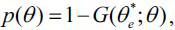 his DI application is approved, and he receives b + d units of consumption. Otherwise, his consumption will be b , which is the combined value of unemployment insurance and possible home production.
b. Government’s Problem
Given the policy rule {p(θ), t, d, b} , workers make optimal decisions as to whether to apply for DI and participate in the labor market. With our assumptions about preferences, we know that the optimal solutions will be cut-off rules. We denote θd as the threshold that makes workers indifferent with regard to receiving DI or being employed: u(y − t) − θd = u(b + d). Similarly, θb solves u(y − t) − θb = u(b).24 Combining the two definitions, we find that θd < θb. Therefore, we can classify workers into three groups according to their optimal choices: workers who always work ( θ < θd ), workers who apply for DI but work if denied ( θd < θ < θb ), and workers who apply fort DI and opt out of the labor market if denied ( θ > θb ).
At this stage, we expand the basic model by introducing additional heterogeneity. The underlying work capacity distribution F(θ) is common, but G(θe | θ) varies by type: G(θe | θ) < Gj(θe | θ) for i < j. This assumption means that if the government applies the common DI award rule θ*, then for same underlying work capacity, the approval rate of type-i will be higher than that of type-j.
If the government still applies universal criteria, θ* for all, the maximization problem is
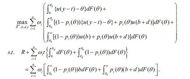
Taking the first-order conditions with respect to θ*, we find that the type-specific trade-offs are weighted using the corresponding population size:

The solution to this maximization is worse than the solution to the more generalized
maximization problem with type-dependent award rule  With the type-dependent rule, we can always find two types below and above the aggregate
mean θ over (θd,θb) interval and improve the welfare by means of redistribution across types.
With the type-dependent rule, we can always find two types below and above the aggregate
mean θ over (θd,θb) interval and improve the welfare by means of redistribution across types.
2. Welfare Analysis
Here, we initially adjust the model environments to calibrate the underlying parameters based on data from South Korean non-college graduates and use the calibration results to conduct a policy analysis.
a. Functional Form Assumptions
Work capacity θ follows an exponential distribution F(θ) = 1 − exp(−γθ) with θ ∈ [0,∞]. The DI award rule is based on medical condition θe, which is correlated with the true work capacity θ such that (θe) = hi(θ) + ε , where ε is the standard measurement error following a normal distribution. The function hi(θ) reflects possible systematic differences in the relationship between θe and θ for type-i workers. G(θe | θ) denotes the cumulative density of θe given θ for type-i.
Individuals have a constant-returns-to-scale (CRRA) utility function over consumption
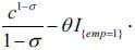 Once approved, workers receive DI independent of their employment status. Thus, given
our utility function, it is always optimal to apply DI. Using the definitions of θd and θb, workers are categorized into three groups according to their optimal labor market
behaviors: (i) those who apply DI and work regardless of the outcome, (ii) those who
apply DI and work only when they are rejected for DI, and (iii) those who apply DI
and do not work when their DI application is rejected.
Once approved, workers receive DI independent of their employment status. Thus, given
our utility function, it is always optimal to apply DI. Using the definitions of θd and θb, workers are categorized into three groups according to their optimal labor market
behaviors: (i) those who apply DI and work regardless of the outcome, (ii) those who
apply DI and work only when they are rejected for DI, and (iii) those who apply DI
and do not work when their DI application is rejected.
b. Data Moments and Calibration
We construct calibration moments using the 9th wave of KLIPS on disability. To do this, we initially categorize the sample with government-registered disabilities into four groups: DI status and two physical intensity levels of pre-disability occupation, denoted by high ( H ) and low ( L ). Using the average intensity among high school graduates as the cut-off, we find that 68% of the population is considered as type- H . With these two characteristics, the observed labor market statistics are as follows:
TABLE 18
MOMENTS
Note: Table 18 reports the moments of the sample according to the medical exam degree (one, two, or three) and the occupational physical intensity level. The sample includes workers aged between 15 and 65 with a high school education and recent employment history. Statistics are weighted using the individual survey weights.
Table 19 summarizes the parameter calibration process. The variable of labor market earnings is normalized to 20. The size of the DI benefit d is taken from the average benefit-to-income ratio among the DI beneficiaries (National Pension System, 2019). The minimum consumption level b is set to 30% of the median income of households, which is the South Korean poverty line.
The scale parameter γ for capacity distribution F(θ) and the DI standard θ* are calibrated to match the aggregate share of the population with medical degrees 1–3 (1.21%) among workers with less than a college education. Assuming that type-L is the baseline with θe = θ, we parameterize hH(θ) = αθ. We find that, to be consistent with the moments, the award rule systematically underestimates disutility from work for type-H workers, i.e. that their observed medical condition is less severe (α < 1). The current model is abstracting other crucial heterogeneities (such as the education level and wealth) that may affect the labor supply decision, and including these elements would deliver a better prediction at a magnitude of α.
c. Counter-factual Experiments
Given the current DI policy, the welfare of type-i workers consists of three parts:
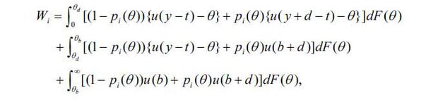
and the aggregate welfare is the weighted average of Wi with the corresponding population share 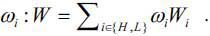 We now compare the welfare implications of alternative DI, focusing on the case in
which the screening process for type-H improves. We can consider this experiment as a case where the South Korean government
factors in work experience and skill sets when evaluating θ, along with medical conditions.
We now compare the welfare implications of alternative DI, focusing on the case in
which the screening process for type-H improves. We can consider this experiment as a case where the South Korean government
factors in work experience and skill sets when evaluating θ, along with medical conditions.
To make the comparison reasonable, we assume that both policies must be budget-neutral.25 Total spending cannot exceed the expenditures from the benchmark analysis, and any additional spending must be financed with lump sum tax t. This results in a moderate increase in taxes, meaning that employed workers pay around 0.5% additionally as income tax. These results are presented in Table 20. Under the new DI program, type-H workers face a less strict disability standard, whereas that of type-L becomes tightened. This results in a decline in employment by 10 pp.
TABLE 20
POLICY EXPERIMENTS
Note: Table 20 compares the economies under the current DI programs to the Vocational Grids.
V. Conclusion
This study examines the relationship between labor market outcomes and individuals’ health status, taking into account occupational requirements. Applying a PCA to O*NET measurements of physical ability, we construct an index of the physical intensity of an occupation and use it to quantify the role of occupation in labor market outcomes by health status.
Our estimation is based on longitudinal South Korean panel data. Using a South Korean household survey has several advantages when studying the relationship between health and occupation. First, unlike most advanced countries, South Korea has a very strict DI program. The share of DI recipients is 1.1% among the working-age population, compared to the OECD average of 6%. Furthermore, the South Korean DI program evaluates its applicants based solely on medical conditions. Thus, the award criteria are independent of the applicants’ occupation histories, unlike in other advanced countries, which consider possible vocational limitations due to disabilities. Moreover, the continuation of the DI benefit is independent of the labor market status of the recipient. These institutional features help us to examine the interplay between occupational characteristics and health shocks in the labor market, alleviating the potential bias caused by DI.
Our analysis shows several interesting results. First, working in a highly physically intense occupation tends to reduce employment rates after the onset of disability, suggesting that vocational consideration would be a reasonable policy to mitigate negative income risks. When we divide the sample by gender, we find that the baseline results remain the same for both groups, although female workers are more responsive. However, when we divide the sample by age, we find that workers below age 45 remain in the market, regardless of their previous occupational characteristics. We also find that younger workers are more likely to switch occupations after the onset of disability. This endogenous response against health shocks tends to be directed, such that workers switch to less demanding occupations. In contrast, all else being equal, exiting the labor market is more common when individuals have accumulated relatively more occupational experience.
Overall, our results suggest that having occupational requirements on physical abilities is important with regard to the labor market outcomes of the disabled. Individuals with less demanding occupational requirements are more apt to be employed, thus remaining in the same occupation. Hence, these workers are subject to lower income risks than are workers with physically demanding occupations. However, as the results suggest, not all individuals with the same occupation face the same risks. Some workers exit the labor market, while others switch to alternative occupations. Understanding the relationship between health requirements and other job skills helps us to understand these varying responses.
Appendices
APPENDIX
A. Data Appendix
In this section, we provide further details of the data construction process used for our empirical analyses.
1. Linking the Occupational Codes
We match the occupation-level characteristics surveyed by the U.S. Department of Labor to a South Korean panel dataset by linking the two country-specific occupational classifications using the International Standard Classification of Occupation (ISCO). The following paragraphs describe the detailed procedure that matches the ISCO with the country-level occupational codes.
a. The International Standard Classification of Occupation (ISCO)
Since 1949, the International Labour Organization (ILO) has provided a comparable list of occupational classifications called the International Standard Classification of Occupation (ISCO). The ISCO categorizes the list of occupations using four layers of occupational classifications. First, the finest occupational descriptions are available for 436 occupations, where each occupation is assigned a four-digit number. Further, two additional layers of occupational classifications group a set of four-digit occupations into 130 cases with three-digit numbers (minor classification) and 43 cases with two-digit numbers (sub-major classification). Finally, these occupations are linked to ten major categories of occupations. Table A1 summarizes the structure of the most recent ISCO, which was released in 2008.
TABLE A1
STRUCTURE OF ISCO-08
Note: Table A1 shows the structure of ISCO-08. Numbers are the sub-classification counts associated with each major classification.
b. The Korea Standard Classification (KSCO)
The South Korean Statistics Department (KOSTAT) provides a list of occupations called the Korea Standard Classification (KSCO) to collect and compare occupation-related data consistently. Analogous to the ISCO, the KSCO adopts a four-layer system of occupational classifications over 400 occupations (Table A2), and eight out of ten major classifications in the KSCO share definitions identical to those of ISCO-08. The other two categories can also be linked by either merging or dividing two major classifications of ISCO-08.26
TABLE A2
THE STRUCTURE OF THE 6TH KSCO
Note: Table A2 shows the structure of the 6th KSCO. Numbers are the sub-classification counts associated with each major classification.
The similarities between the two classifications help us to link the KSCO into ISCO-08. KOSTAT provides the official crosswalk table between ISCO-08 and the 6th KSCO.27 According to the crosswalk table, 318 out of 426, or 74.6% of four-digit occupations have a one-to-one relationship from the KSCO to ISCO-08 (KOSTAT, 2018) The remaining 108 occupations of KSCO have multiple matched occupations in ISCO-08 (Table A3). As a result, we have 596 possible combinations between ( 318 + 72× 2 +19 × 3 + 12 × 4 + 2 × 5 + 2 × 6 +1 × 7 ) the 6th KSCO and ISCO-08. It is important to note that this does not imply that there are 318 unique ne-to-one matches. Different occupations in the KSCO (called A and B ) may be separately linked to one occupation x in ISCO-08, generating two one-to-one matches A: x and B : x . As a result, inverse matching from ISCO-08 to the KSCO shows different outcomes.28
TABLE A3
LINKAGE BETWEEN THE 6TH KSCO AND THE ISCO-08
Note: Table A3 reports the results of the matching of the 6th KSCO to ISCO-08 using the crosswalk table provided by KOSTAT.
c. The U.S. Occupational Classification
Although the U.S. Standard Occupational Classification (SOC) was recently modified in 2018, the most recent crosswalk table between ISCO-08 and the SOC is based on the 2010 version of the codes. Thus, we match ISCO-08 with the SOC in terms of four-digit level based on the 2010 SOC. As the Bureau of Labor Statistics (BLS) uses 23 major classifications, the resulted linkage from ISCO-08 to the 2010 SOC more frequently involves a merging of multiple occupations. Nonetheless, 67.5% of the occupations can be represented by the matching of an occupation in ISCO-08 with three or fewer occupations in the 2010 SOC (Table A4).29
TABLE A4
LINKAGE BETWEEN ISCO-08 AND THE 2010 SOC
Note: Table A4 reports the match results of the 2010 SOC to the ISCO-08 using the crosswalk table provided by the BLS.
d. Linking the Occupational Codes across Countries
Here, we describe how we linked the KSCO and the 2010 SOC using ISCO-08. As shown in Tables A3, 318 out of 426 (74.6%) occupations in the KSCO form a unique match with ISCO-08, and 409 of 426 (96%) occupations in the KSCO can be described with three or fewer occupations in ISCO-08. Based on the results in Tables A3 and A4, we link all possible matching combinations of ISCO-08 and the 2010 SOC to each occupation in the KSCO.
TABLE A5
LINKAGE BETWEEN THE 6TH KSCO AND THE 2010 SOC
Note: This table reports the results of the matching of the 6th KSCO to the 2010 SOC via ISCO-08 using the official crosswalk tables provided by KOSTAT and the BLS. There is no match from ISCO-08 (5343) to the SOC, leaving one of the KSCO codes (5301) unmatched.
B. A Model without Heterogeneity
The government’s objective function is
where R represents additional resources available. Setting the Lagrangian problem for equation (A1), we obtain the following four first-order conditions:

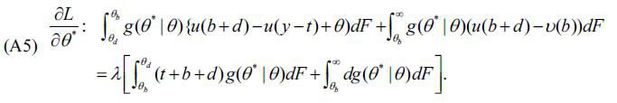
The first two conditions show that it is optimal to provide partial insurance due to moral hazard concerns: y − t > b + d.30 equation (A5) states that at the optimum criteria for disability θ*, additional welfare changes among DI beneficiaries must be equal to the corresponding financial costs. We denote the net welfare of marginal DI recipients switching from non-employment as Δd ≡ u(b + d) − u(b) − d λ and, similarly, the net welfare change from employment as Δe + θ ≡ u(b + d) − u(y − t) + θ − λ(t + b + d). Using these notations, equation (A5) can be written as

The last term of the equation above is strictly positive; thus, at the optimum, the
first two terms have opposite signs. Assuming standard concave utility functions,
we can show that 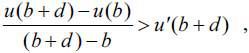 where u′(b + d) ≥ λ. Therefore, u(b + d) − u(b) > λd and Δd is strictly positive. This result implies that the optimal DI cutoff is set at the
level with a positive net welfare gain for those who have no work capacity. The optimality
condition in the more generalized setup is the weighted average of equation (A6) with
its population size.
where u′(b + d) ≥ λ. Therefore, u(b + d) − u(b) > λd and Δd is strictly positive. This result implies that the optimal DI cutoff is set at the
level with a positive net welfare gain for those who have no work capacity. The optimality
condition in the more generalized setup is the weighted average of equation (A6) with
its population size.
Notes
This paper is revised version of Rhee, 2019, “Disability Insurance Eligibility Reform and Its Implications,” the KDI working paper (in Korean). Rhee thanks Dongseok Kim (the editor), two anonymous referees, Jiwoon Kim, and Junghyun Kwon for their helpful comments. Choran Jeon provided excellent research assistance.
These patterns can be found in other countries too. For instance, Campolieti (2002) and Cai and Kalb (2005) use Canadian and Australian datasets, respectively, to show a decline in labor force participation after the onset of disability. Kwon (2018) finds similar results among South Korean males.
Recent studies of the role of occupational characteristics in labor market outcomes expand this framework by estimating the labor transitions, summarizing occupations as sets of tasks that require multidimensional skills (e.g., see Lise and Postel-Vinay, 2019 and Guvenen et al., 2020).
The US Social Security Administration (SSA) applies more generous criteria to older, less educated, non-English-speaking applicants because they are expected to have greater difficulty in developing skill sets for new occupations (Wixon and Strand, 2013).
In terms of the scale of recipients, only 1.1% of the South Korean working-age population is currently enrolled as DI recipients. In other OECD countries, 6% of their working-age populations receive DI payments on average (source: https://data.oecd.org/healthres/health-spending.htm).
Indeed, about 37% of working-age individuals registered as disabled for work-related events are currently employed in South Korea (source: disability survey of KLIPS, 9th wave).
The lower age bound for eligibility is 18, and the upper bound gradually increases depending on the applicant’s birth year: age 61 for those born in the years 1953—1956, age 62 for those born in the years 1957—1960, age 63 for those born in the years 1961—1964, age 64 for those born in the years 1965—1968, and age 65 for those born after 1969.
The categories are vision, hearing, speech, arm/leg/spine, mental disorders, respiratory disorders, cardiovascular system, digestive system, liver disease, hematological disorders, abdomen/pelvic organs, facial disorders, and cancer.
The average monthly income for an urban household of one in the year 2019 is 2,545,147 Korean won, which is 4.24 times greater than 600,000 Korean won.
The Listing of Impairments (also known as the Blue Book), which contains the type of disability with sufficient medical conditions for DI eligibility, is available on the SSA webpage (Listing of Impairments).
Since 1985, DI awards based on residual functional capacity increased threefold (Michaud et al., 2018). In 2010, 13.6% of applicants received DI for proving sufficiently severe medical conditions, and 16.8% received DI after the residual capacity evaluation (Wixon and Strand, 2013).
Chen and van der Klaauw (2008) exploit this institutional feature to estimate the labor supply distortion created by DI using a regression discontinuity method. Their results suggest that DI recipients’ labor supply would have increased by 20 pp had none received benefits.
These are the level and importance of the following nine characteristics: dynamic flexibility, dynamic strength, explosive strength, extent flexibility, gross body coordination, gross body equilibrium, stamina, static strength, and trunk strength. The importance score reflects how relevant it is with regard to performing the main tasks of an occupation, while the level score indicates the difficulty required when performing occupational tasks.
Indeed, the overall Kaiser–Meyer–Olkin measure of sampling adequacy is 0.933, indicating that our sample is appropriate for a PCA (Kaiser, 1974).
A similar approach can be found in Lise and Postel-Vinay (2019), who map more than 200 O*NET job descriptors into three skill requirements— mathematical, mechanical, and social skills —and estimate a structural job search model of multidimensional skills. Guvenen et al. (2020) process multiple test scores available in NLSY79 into three ability measures for individuals (math, verbal, and social skills) using a PCA and gauge the degree of mismatch in the US labor market.
Multiple matches mostly occur in occupations in information technology and healthcare, where the SOC adopts more granular definitions, whereas the KSCO and ISCO use broader classifications.
The current health evaluation and relative evaluation results are strongly correlated ( ≈ 0.8 ).
Specifically, the survey asks whether a respondent has experienced difficulties in job-related activities owing to his health status.
We conduct robustness analyses using alternative strict definitions of disability and find qualitatively similar results. The robustness analyses are reported in Section 4.2.
The coefficient estimate for physical intensity is 0.00039 with 95% CI [-0.0030,0.0038] and are thus omitted for brevity.
Under the current DI program, the benchmark economy is spending 12.20% of average labor productivity for social insurance. Because we are analyzing only high school graduates, we may consider this result as redistribution toward high school graduates.
Instead of “service and sales workers” in ISCO-08, the KSCO adopts the two separate categories of “service workers” and “sales workers.” While ISCO-08 has two separate categories for “professionals” and “technicians and associated professionals,” the KSCO combines the two categories into “professionals and related workers.”
While its most recent 7th revision was introduced in 2017, we decided to use the 6th KSCO as our main classification because the panel dataset for the main analysis is reported based on the previous occupational codes.
For instance, the KSCO separately labels “Company Grade Officers” and “Field Grade Officer or Higher Ranks,” but ISCO-08 labels both occupations as “Commissioned Armed Force Officers.”
 is the weighted average of the inverse marginal utilities. Because the RHSs of the
first-order conditions are non-negative, u′(b)>u′(b+d)≥λ or
is the weighted average of the inverse marginal utilities. Because the RHSs of the
first-order conditions are non-negative, u′(b)>u′(b+d)≥λ or 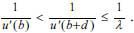 Therefore, it must be the case that
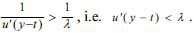
References
, , , & (2019). Disability Benefits, Consumption Insurance, and Household Labor Supply. American Economic Review, 109, 2613-2654, https://doi.org/10.1257/aer.20151231.
(2013). The “Task Approach” to Labor Markets: An Overview. Journal for Labour Market Research, 46, 185-199, https://doi.org/10.1007/s12651-013-0128-z.
(2002). Disability and the Labor Force Participation of Older Men in Canada. Labour Economics, 9, 405-432, https://doi.org/10.1016/S0927-5371(02)00051-9.
, & (2008). The work disincentive effects of the disability insurance program in the 1990s. Journal of Econometrics, 142, 757-784, https://doi.org/10.1016/j.jeconom.2007.05.016.
, & (1995). Economic Aspects of Optimal Disability Benefits. Journal of Public Economics, 57, 1-23, https://doi.org/10.1016/0047-2727(94)01435-Q.
(2005). The Effects of Health, Wealth, and Wages on Labour Supply and Retirement Behaviour. Review of Economic Studies, 72, 395-427, https://doi.org/10.1111/j.1467-937X.2005.00337.x.
, , & (2015). The U-Shapes of Occupational Mobility. Review of Economic Studies, 82, 659-692, https://doi.org/10.1093/restud/rdu037.
(1974). An Index of Factorial Simplicity. Psychometrika, 39, 31-36, https://doi.org/10.1007/BF02291575.
, & (2009a). Occupational Mobility and Wage Inequality. Review of Economic Studies, 76, 731-759, https://doi.org/10.1111/j.1467-937X.2009.00535.x.
, & (2009b). Occupational Specificity of Human Capital. International Economic Review, 50, 63-115, https://doi.org/10.1111/j.1468-2354.2008.00524.x.
, & (2018). Measuring the Effects of Employment Protection Policies: Theory and Evidence from the Americans with Disabilities Act. Labour Economics, 54, 116-134, https://doi.org/10.1016/j.labeco.2018.08.001.
, , & (2007). Consumer Bankruptcy: A Fresh Start. American Economic Review, 97, 402-418, https://doi.org/10.1257/aer.97.1.402.
, & (2015). Disability Insurance and the Dynamics of the Incentive-Insurance Trade-Off. American Economic Review, 105, 2986-3029, https://doi.org/10.1257/aer.20110108.
, , & (2018). Vocational Considerations and Trends in Social Security Disability. Journal of the Economics of Ageing, 11, 41-51, https://doi.org/10.1016/j.jeoa.2016.12.001.