
Korea’s Demographic Transition and Long-Term Growth Projection Based on an Overlapping Generations Model
Abstract
This paper employs an Overlapping Generations Model to quantify the impacts of Korea’s demographic transition toward an older population on the total output growth rate. The model incorporates the projected population through 2060 according by Statistics Korea. The effects of the low fertility and increased life expectancy rates are studied. The model is considered suitable for analyzing the effects of demographic changes on the Korean economy. Under the assumption that the TFP growth rate will not slow considerably in the future, remaining at 1.3% per annum, the gross output growth rate of the Korean economy is projected to slow to 1.1% per annum in the 2050s, from 4.0% in the 2000s. The shrinking workforce due to the decline in fertility plays a significant role in the deceleration of the Korean economy. The increased life expectancy rate is expected to mitigate the negative effect, but the magnitude of its effect is found to be limited.
Keywords
Computable General Equilibrium Models, Life Cycle, Aggregate Supply, Population Aging
JEL Code
C680, E210, J110
I. Introduction
Korea’s population structure is rapidly changing. According to Statistics Korea, the total population is projected to peak at 52.1 million in 2030 and then to fall to 43.9 million by 2060. In particular, the working-age (15~64) population, which largely determines the size of the labor force, is forecast to shrink at an accelerated rate due to a persistently low fertility rate, dwindling to 21.8 million by 2060; a mere 59% of its peak of 37.0 million in 2016. Roughly speaking, the working-age population will decrease by approximately 0.3 million, or 1~2% per annum, for the next 45 years. On the other hand, as life expectancy continues to improve, the old-age (aged 65 and over) population is projected to surge to 17.6 million in 2060 from 5.4 million in 2010. Consequently, the old-age dependency ratio is also expected to rise to 80.6% from merely 15.2% as of 2010. Indeed, Korea’s demographic structure is changing at an alarming rate by international standards. In terms of the old-age dependency ratio, Korea is projected to become one of the most aged countries by 2050 among OECD member countries, as shown in Figure 1.
FIGURE 1.
A PROJECTION OF THE AGED DEPENDENCY RATIO FOR OECD COUNTRIES
Note: The horizontal axis indicates the old-aged dependency ratio in 2014. The vertical axis indicates the old-aged dependency ratio in 2050.
Source: OECD. Stat.
The rapid demographic transition is expected to affect the economy through various channels. Due to the ongoing low fertility rate, the size of the workforce will decline and lower the growth potential. From a household perspective, the continued increase in longevity, however, will alter economic decisions about consumption-saving and working hours, among others. Specifically, longer life expectancy tends to increase the incentives to work unless the retirement age is prolonged in proportion. Moreover, lower fertility implies that fewer children will be present in households during working years, and this acts to reduce consumption before retirement. These changes in household behavior could positively affect the economy through aggregate labor supply and capital accumulation channels.
In this paper, we build an overlapping generation general equilibrium model to analyze the effects of Korea’s demographic changes on GDP growth potential to the year 2060.1 Focusing on GDP to measure a country’s well-being may not be appropriate, especially for countries experiencing rapid population aging. However, it is still an important measure for Korea as a sharp decline in the GDP growth rate exacerbates, for instance, long-term fiscal and generational redistribution issues due to a sharp increase in welfare spending.
The demographic transition of the model economy closely follows the historical data and official projections published in 2011 by Statistics Korea. The model economy is populated with households that face mortality risks and may live to a maximum age of 100. Households have one male and one female adult and a varying number of children. To reflect the possibility that the female workers may play a greater role in the labor market in the future due to the scarcity of labor, an endogenous female labor supply response is considered in the model economy. As a way of modeling the endogenous female labor supply, we assume that adult members jointly choose how much to work and how much to consume (or save) to maximize the household life-time utility. For the demographic transition, two distinct sources of exogenous variation are considered: changes in the fertility rate and changes in the survival probability. In addition to the changes in the volume of the labor force caused by the interaction between fertility rates and survival probabilities, households’ endogenous responses, such as work hours and consumption-saving decisions are considered.
Our objective is to assess the effects of demographic changes on the macro economy in the coming decades. The endogenous responses of the model economy to exogenous variations in the demographic variables and the changes in total factor productivity are reasonably successful in reproducing the historical path of labor growth, capital accumulation, and GDP growth. Therefore, the model is considered suitable for analyzing the effects of the aforementioned demographic changes on the Korean economy. Under the assumption that the TFP growth rate will not decelerate much in the future, remaining at 1.3% per year, the growth rate of the Korean economy is projected to decelerate to 1.1% per annum in the 2050s from 4.0% in the 2000s. A shrinking workforce plays a significant role in the slowdown of the Korean economy, although the increased life expectancy is expected to mitigate the negative effects, albeit to a limited degree.
Analyzing the demographic effects on the future Korean economy in the framework of the Overlapping Generations model is not unprecedented. For example, Hong (2007) studies macroeconomic impacts of an aging population in Korea using an Auerbach-Kotlikoff type of model; Lee and Moon (2013) analyze the long-run and transitional impacts of different fiscal rules on the future path of the Korean economy; Shin and Choi (2015) develop a model in which the accumulation of human capital is endogenously determined and project the long-term economic growth.
These studies are, however, silent with regard to how much the model economies can explain the historical paths of macro variables, casting doubt therefore on the validity of the models when used to assess the effects of demographic changes on the macro economy in the coming decades. In addition, to the best of our knowledge, this paper is the first to consider the role of the female labor supply for the Korean economy in the coming decades in the overlapping generations model framework. As Korea’s female labor participation rate is one of the lowest among OECD member countries, there appears to be sufficient room for improvement regarding the female labor supply. As the size of the labor force shrinks, the female labor supply is expected to increase as a result of market forces given the scarcity of labor. Therefore, it is important to quantify the contributions of the female labor supply on the aggregate labor supply to assess the effects of demographic changes on the macro economy for the Korean economy.
For Japan’s economy which is also experiencing drastic demographic changes, similar to those in Korea, Chen, Imrohoroglu, and Imrohoroglu (2005, 2007) and Braun, Ikeda, and Joines (2009) analyze the effects of demographic changes on saving rates and show that a demographic transition is a key determinant in the long-run swing in Japan’s saving rates.
This paper is organized as follows: Section II specifies the model economy; Section III calibrates the model based on various macro and micro datasets; Section IV evaluates the model’s ability to explain the observed macro data and reports our baseline projections for the Korean economy; Section V presents counter factual exercises; Section VI concludes the paper.
II. The Model Economy
Our theoretical model is a standard life- cycle, overlapping generations model. The basic structure of the model economy is adapted from Braun, Ikeda, and Joines (2009), especially for the population and household structure.
A. Demographic Structure
Time t is discrete and the model period is one year. Individuals who face mortality risks
in each period may live up to J periods such that J birth cohorts are alive in the economy in any period t. Let N j,t denote the population of age j in period t. The population of each cohort in period t is described by Νt, which is a J × 1 vector of which the elements are N j, t. The number of the total population in period t is given by  .
.
The population of each cohort evolves over time as follows:
N1,t+1 = (1+n1,t+1)N1,t.
Nj+1,t+1 = Ψj,tNj,t, 1 ≤ j ≤ J−1
Nj+1,t+1 = 0.
where n1, t +1 denotes the growth rate of the population of age 1 in period t +1, referred to as the fertility rate hereinafter. ψ j,t denotes the conditional probability that an individual aged j in period t survives to period t +1. We assume that J is one hundred and that ψ j,t is zero. We assume further that the same number of males and females are born during each period and that they share identical conditional survival probabilities. That is, the survival probabilities only differ by birth cohorts.
The model economy is populated with households that consist of one male adult, one female adult, and varying number of children under the age of 20. At the age of 21, one male and one female form a household. Hence, the number of households aged j in period t is denoted as N j,t / 2, for j ≥ 21. Each household exits from the economy when a mortality shock arrives.
Households have varying numbers of children. Specifically, let mj,t be the number of children born to a household aged j in period t. As time passes, the number of children increases, as does the size of the household η j,t. When the children become 21, they separate from the household to form their own households and the size of the household decreases. Accordingly, the size of a household evolves over time, as follows:

B. Household’s Problem
A household is a unit that makes independent economic decisions concerning consumption-saving and the labor supply, among athers. Each household participates in the labor market at the age of 21 and retires at the age of JR. 2 We refer to a household aged j in period t as belong to the kth cohort. Note that age, time, and cohort indices are not independent given that k = t − j +1. We notate the model economy with only time and age indices unless it is absolutely necessary to do with the cohort indices.
We assume that there exists a household that represents the average characteristics of the kth cohort. The lifetime utility for this representative household of kth cohort is assumed as follows,

where cj,t denotes the consumption of household aged j in period t, and hMj,t and hFj,t denote the hours of work for the male and the female members, respectively. We assume that the lifetime utility is time-separable and that the discount rate is identical for all cohorts. β denotes the preference discount rate. πj,t is the unconditional probability of surviving from birth to age j in period t and is calculated as follows: πj,t = ψj−1,t−1πj−1,t−1,π1,t = 1 for all t.
We assume the following instantaneous utility function:

The utility function is separable between consumption and leisure. This utility function was chosen to support a balanced growth path. The parameter γ denotes the intertemporal substitution elasticity of leisure.
We expect that the female labor supply will play a greater role in the coming decades as the working-age population decreases. One channel through which the female labor supply will increase is the decline in the household size. As the average household size over the life cycle decreases, so will the relative value of household production to market work, which results in an increase in the female labor supply. To accommodate this channel, we assume that the disutility from market work by the female household member is an increasing function of the household size.
Each household has two adult workers: one male and one female. Workers have different labor market productivity values according to gender and age. Let ϵMj be the time-invariant productivity of an aged - j male worker and ϵFj,t be the productivity of an aged - j female worker in period t. When the household aged j in period t supplies hMj,t, hFj,t hours to the labor market, it supplies 𝟄MjhMj,t + 𝟄Fj,thFj,t units of efficiency labor and earns wt𝟄MjhMj,t + wt𝟄Fj,thFj,t, where wt denotes the market wage rate for an efficiency unit of labor in period t.
A household enters the economy without assets. Borrowing against the future labor income is not allowed. Let rt denote the market interest rate, which is rate of return on savings. When a household exits from the economy due to mortality shock, it leaves its unconsumed assets to its children’s generations. However, the household does not take into account the children’s utility; therefore all of the bequests in this economy are unintended. Likewise, the children inherit assets from their parents’ generations. Let bj,t be the amount of transfer income that the representative household aged j in period t receives from their parents’ generations.
A household’s decision problem is formulated recursively and Bellman’s equation for a representative household of age j in period t is given as follows:
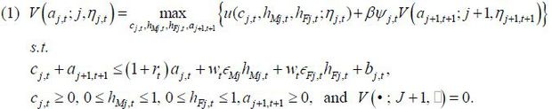
The decision rules that solve this problem are denoted as cj,t = c(j,t), hMj,t = hM(j,t), hFj,t = hF(j,t) and aj+1,t+1 = a'(j,t).
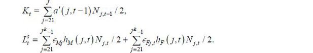
The aggregate supply of capital in period t + 1,  , is determined by the households’ decisions on savings. In order to calculate the
aggregate supply of capital, we need to specify how unintended bequests are distributed
to living households. The aggregate supply of aggregate capital in period t + 1 is determined by the saving behaviors of the representative households in period
t. The amount of assets that the representative household aged ݆j in period t saves is a'(j,t). This household survives in period t + 1 with a probability of ψ j,t or exits from the economy with a probability of (1 − ψ j,t). If a mortality shock arrives, we assume that the assets, including the return on
savings are transferred to their children’s generations as an accidental bequest at
the end of period t + 1. In other words, the inheritors receive (1 + rt+1)a'(j,t) in the period of t + 1. The total amount of these unintended bequests in the model economy in period
t + 1 is
, is determined by the households’ decisions on savings. In order to calculate the
aggregate supply of capital, we need to specify how unintended bequests are distributed
to living households. The aggregate supply of aggregate capital in period t + 1 is determined by the saving behaviors of the representative households in period
t. The amount of assets that the representative household aged ݆j in period t saves is a'(j,t). This household survives in period t + 1 with a probability of ψ j,t or exits from the economy with a probability of (1 − ψ j,t). If a mortality shock arrives, we assume that the assets, including the return on
savings are transferred to their children’s generations as an accidental bequest at
the end of period t + 1. In other words, the inheritors receive (1 + rt+1)a'(j,t) in the period of t + 1. The total amount of these unintended bequests in the model economy in period
t + 1 is

The total amount of the unintended bequest inherited by the living households can be denoted as

With this timing of the transfer process, the aggregate supply of capital in period
t + 1, , can be calculated as the total amount saved by the representative households in
period t. That is

The aggregate supply of labor in period t is

C. Firm’s Problem
In the model economy, there exists a representative firm which produces output Yt by combining capital Kt and labor Lt using a constant return to-scale Cobb-Douglas production function in each time period t,

where At denotes the total factor productivity in period t and α is the output elasticity of capital. The aggregate labor Lt is measured in units of efficiency. We assume that the markets for the factors of production and the market for goods are competitive.
The firm’s profit maximizing problem can be stated as follows,

where  and
and  denote the demand for labor and the demand for capital, respectively, and δt denotes the depreciation rate of capital in period t. Then, and satisfy the following first-order profit maximizing conditions:


D. Capital Flows
We assume that the model economy is closed such that the rate of return on capital is determined in the domestic market. We rely on the empirical findings of Feldstein and Horioka (1980), which show that the correlation between the investment rate and the savings rate is close to one in the long run given this assumption. Considering that other economies also have aging populations, the trend in the future capital flows will be determined by the relative speed of Korea’s demographic transition. It may be beneficial to model a multi-country large-scale Overlapping Generations Model to account for the effects of the world-wide demographic transition on global rates of return on capital. Examples include Attanasio, Kitao, and Violante (2007) and Krueger and Ludwig(2007). The effects of Korea’s demographic transition on the Korean economy can then be analyzed in a single framework under the open economy assumption. However, doing so world be beyond the scope of this paper, and we therefore limit our model to the closed economy assumption.
D. Definition of Recursive Competitive Equilibrium
Let St = {n1,t, ψt, ηt, At, δt} be the aggregate state of the economy in period t, where ψt = {ψ1,t, ψ2,t,⋯,ψj,t} is the vector of conditional survival probability in period t and ηt = {η1,t, η2,t,⋯,ηj,t} is the size of the representative household in period t. We assume that the economic agents in the economy perfectly foresee the entire path of the state of the aggregate economy, {St}.
Given the path of the aggregate state of the economy, the equilibrium of the economy consists of the household’s value function V(aj,t; j, ηj,t); the associated decision rules c(j,t), hM(j,t), hF(J,t) and a'(j,t); the sequence of the aggregate factor inputs {Kt,Lt}; and the sequence of the factor prices; {wt} and {rt} such that
1. Given the path of the factor prices, the household value function and the decision rules solve the household’s dynamic problem (1).
2. Given the path of the factor prices, (Kt, Lt} denotes the solution to the representative firm’s profit maximization problems (2) and (3).
3. The factor markets clear: for all t,
4. The goods market clears: for all t, 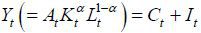 , where
 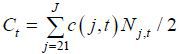 and It = Kt+1 − (1 − δt)Kt.
5. The amount of transfer income that living households receive is in line with the
amount of accidental bequests: for all t,  .
.
Balanced Growth Path
In order to quantify the model economy, we must specify the characteristics of the balanced growth path to which the model economy converges. We assume, in the end, that the net fertility rate and the conditional survival probabilities converge and become constant:
 for 1 ≤ j ≤ J and all t ≥ T*.
After passing J periods after these conditions are satisfied, we have

In other words, the growth rate of the total population is equal to the net fertility rate, and the age distribution of the population becomes stationary.
We assume that the growth rate of total factor productivity converges in the end.
That is  for all t ≥ T*.
Suppose that a stationary population distribution is achieved and that the growth rate of total factor productivity is constant over time. In such a case, the stationary recursive competitive equilibrium is recursive competitive equilibrium in which the following characteristics are satisfied. For all t, the consumption and savings of the representative household increase proportionally and the supply of labor remains constant:
 ,
,  ,
,
 ,
,  for all j and t ≥ T*,
Where  .
.
In consequence, the market prices are determined as follows:
rt = r*,  for t ≥ T* , where
  .
.
III. Calibration
A. Demographic Transition
We calibrate the model economy with information for the period between 1991 and 2010. Then, we simulate and analyze the model economy through to the year 2060, for which the official population projection by Statistics Korea is available. The demographic transition of the model economy mimics the projection. Assumptions about fertility and survival probabilities are required to produce the age distribution of the population at each date. The net fertility rates are calculated to match the growth rate of the one-year-old population until the year 2060. To solve the model economy quantitatively, we need information beyond 2060. Between 2060 and 2100, the net fertility rates are drawn from the UN’s population projection data. After 2100, they are assumed to be fixed at zero. Through 2060, the conditional survival probabilities are drawn from the life tables projected by Statistics Korea. Because the projected life tables are in five-year periods, the probabilities for the interim periods are approximated by linear interpolation. After 2060, the survival probabilities remain fixed at the 2060 levels. Under the assumptions specified above, the population distribution reaches a steady state in 2180, wherein the population growth rate is zero percent and the age distribution of the population does not change over time.
The size of the representative household, ηj,t, is constructed in a manner that is consistent with the population projection with simplifying assumptions. The method suggested by Braun, Ikeda, and Joines (2009) is modified to be consistent with our model economy. Regarding the size of a household aged j in period t, as shown in equation (1), we need to construct the number of children born to the household aged j in period t, i.e., mj,t. Let pj,t denote the proportion of children that are born to all females aged j in period t to the total number of children born in period t. The number of children born to all females aged j in period t can then be written as pj,tN1,t. Finally, we determine the number of children born to household aged j in period t with the equation mj,t = pj,tN1,t / (Nj,t / 2), where Nj,t / 2 is the number of households aged j in period t in the model economy.
At this stage, we need to find an empirical counterpart for pj,t. For the years between 1981 and 2014, we can easily calculate pj,t from Statistics Korea’s Birth Statistics data. However, for other years, we need additional simplifying assumptions due to the lack of historical data and projections of pj,t. We assume that mj,t = ftmj, where mj = mj,1981 for the years before 1981 and mj = mj,2014 or the years after 2014. Following Braun, Ikeda, and Joines (2009), we interpret ft as a time-varying shock to aggregate fertility and mj as the time-invariant indicator of the relative number of births in each year of the parents’ life cycles. We calculate ft as follows:

B. Households
Micro estimates of the intertemporal substitution elasticity of leisure, γ, range from 0.1 to 0.7. We choose a value of 0.5 for both male and female workers, which is a widely accepted value for the class of the model economy considered in this paper. We choose the weight parameters for disutility from working BM and BF such that the average number of hours of work is 1/3, respectively, on the balanced growth path.
The preference discount factor β is set such that the average savings rate of the model economy during 1991~2010 matches the average value of the savings rate and investment rate for the same period. Note that we pinned down the average savings rate of the model economy between 1991 and 2010, but the dynamics of these variables are determined endogenously.
Model simulations require initial asset holdings by age in the year 1991. We use Statistics Korea’s Household Asset Survey for 2006 to determine the age-asset distribution in 1991; although this survey was conducted for the year 2006, to the best of our knowledge it is the earliest data publically available. Then, the aggregate wealth of the model economy in 1991 is then rescaled to match the capital-output ratio in 1991, which is 2.6.
The age-productivity profiles by gender are constructed from the data on employment, wages, and weekly hours collected by the Ministry of Employment and Labor for 1993~2014.5 The method suggested by Hansen(1993) is employed to the extract age-productivity profile. Wages are converted to the actual values using the consumer price index. Figure 2 shows the age-productivity profiles by gender. The age-productivity profile for a male worker is normalized to have an average value of one. As reported for most advanced countries, it has an inverted U shape. For male workers, we assume that labor productivity varies with age but that the age-productivity profile itself is invariant over time. Thus, growth in labor productivity for male workers is solely attributed to the total productivity growth in the model economy. The age-productivity profile for a female worker is reported in values relative to those of male workers. For example, the labor productivity rate for female workers aged 40~44 is about 0.8, which is approximately 80% of the average productivity of male worker.
FIGURE 2.
AGE-PRODUCTIVITY PROFILE BY GENDER
Note: Employing the method by Hansen (1993), the numbers are calculated by the author.
We assume that the female age-productivity profile converges to that of their male counterparts over time. Figure 3 shows the female age-productivity profiles calculated for the half periods. The age-productivity for a female worker shows an increase in the sample periods. We assume that this improvement continues until it converges to the male age-productivity profile at the historical speed. What the method suggested by Hansen (1993) recovers is simply the average hourly real wage rate by age group and gender. If the labor market is competitive, the hourly wage rate reflects the true worker’s productivity. However, we recognize well that the hourly wage rate may not truly reflect worker productivity and that the problem may be more complicated if we compare those values between males and females. The difference may reflect such factors as gender discrimination and different levels of experience or education. As labor is expected to become scarce, we expect that the working environment will improve culturally and legally in such a way that female workers will remain in the labor market and the relative difference between male and female workers will disappear gradually in the future. We interpret the convergence of the female age-productivity profile to its male counterpart as a reflection of these changes.
FIGURE 3.
DIFFERENCE IN AGE-PRODUCTIVITY PROFILE FOR FEMALES OVER TIME
Note: Employing the method by Hansen (1993), the numbers are calculated by the author.
C. Other Parameters
The values for the remaining parameters are chosen in line with Cho (2014). The author reports a GDP projection to 2035 employing what is termed “the production function approach.” For the output elasticity of capital, we choose a value of 0.39, which is the capital income share in 2013.6 We assume that the output elasticity of capital is constant over the simulation period. The time series of the depreciation rate is calculated with data pertaining to the aggregate capital stock by the Bank of Korea and the gross real fixed investments of national accounts. The depreciation rate appears to increase from 5.0% to 5.2% during 1990~2014. We project that the value will increase to 5.4% in 2035 and remain constant thereafter.
The historical value of the total factor productivity (TFP) is calculated by the standard growth accounting method. In this paper, the TFP is identified as the Solow residual; thus, different measures of labor and capital input yield different values of the TFP. To maintain consistency with the model economy, we define the labor input as the total number of employees weighted by the age-productivity profiles. For the future values of total factor productivity, we adopted the TFP growth rate from Cho (2014) by 2035 and assume that there is continued growth thereafter at a constant rate of 1.3 percent per annum.7
IV. Results
A. In-Sample Performance of the Model
Our objectives are to project the future path of macro variables and to analyze the effects of the demographic transition on the growth potential of the Korean economy. Before doing so, we examine the in-sample performance of the model economy in this subsection. We compare the simulated aggregate variables with the relevant historical data, in the case employment, the investment rate, and the real GDP growth rate.
Figure 4 shows the aggregate labor growth rate of the model economy and the employment growth rate from the Economically Active Population Survey.8 Also shown in the figure is the growth rate of the population aged 21~64 of the model economy. The employment growth rate exhibits a slow downward trend and short-run fluctuations. The trend in the employment growth rate is well- captured by the growth rate of the population aged 21~64 of the model economy. The employment growth rate was 1.6% per annum in the 1990s and 1.2% per annum in 2000s. For the respective periods, the aggregate labor for the model economy grew by 1.5% and 0.8% per annum. The aggregate labor growth rate of the model also displays a pattern similar to that of the employment growth.
FIGURE 4.
GROWTH RATE OF AGGREGATE LABOR
Note: The working-age is between 21 and 64.
Source: Statistics Korea(1993~2014).
Figure 5 presents the investment rate of the model economy together with the gross savings rate and the gross investment rate. The gross saving rate and the gross investment rate have continued to decline from above the 40% range in the early 1990s to slightly above the 30% range in the early 2010s. This secular decline is well replicated by the model economy, which reflects that the slowdown in the TFP growth and the decline in the growth rate of the working-age population have lowered the demand for investment. As the model investment rate shows a pattern similar to the data, so does the growth rate of capital stock, as presented in Figure 6. However, it was found that the investment boom in the 1990s is not well captured in the model economy. This stems partly from the information assumption that economic agents perfectly foresee the future state of the economy. That is, the investment boom may have been based on optimistic expectations for the Korean economy. However, the economic agents in the model who perfectly forecast the slowdown of the economy do not invest as much as we see in the data for that period.
FIGURE 5.
INVESTMENT RATE
Note: The investment rate and saving rate are measured as proportions to the real GDP by the author’s calculation.
Source: Bank of Korea(1993~2014).
Figure 7 shows the output growth rate of the model and the real GDP growth rate. The model economy exhibits not only a declining trend in the GDP growth rate but also similar short-term fluctuations. This occurs because, over the short term, the responses of the endogenous variables of the model to the variation in the TFP are generally in line with the data. Table 1 presents the growth accounting calculations for the model in ten-year periods. The numbers in the parentheses are growth accounting calculations for the Korean economy drawn from Cho (2014).
TABLE 1
GROWTH ACCOUNTING FOR THE MODEL ECONOMY
Note: The numbers in the parentheses are growth accounting for the Korean economy drawn from Cho (2014).
From approximately 6.7% per annum in the 1990s, the real GDP growth rate has declined to about 4.3% in the 2000s. As is well- known, the contribution of capital accumulation decreased sharply during this period as the TFP growth rate declined and the economically active population growth slowed. Our model economy does not capture the investment boom in the 1990s well. Overall, however, our model economy is considered reasonably successful in replicating the trends in the GDP growth of the Korean economy. Therefore, given the assumptions of a demographic transition and the future path of the TFP, our model economy is expected to yield reasonable responses for macro variables.
B. Baseline Projection
We now use the baseline model to project the future path of the Korean economy. Table 2 presents the long-term growth rate projection up to 2060. Also shown in parentheses is the long-term GDP growth projection for the Korean economy drawn from Cho (2014). As expected, the long-term output growth rate is projected to decline steadily. From about 2.6% per annum in the 2010s, it is projected to be about 1.8% per annum in the 2020s and to decline further to 1.1% by the 2050s.
TABLE 2
GROWTH ACCOUNTING FOR THE BASELINE PROJECTION
Note: The numbers in parentheses are the GDP growth projection in the form of growth accounting for the Korean economy drawn from Cho (2014).
To analyze the factors contributing to this secular decline, we report the results in the form of a growth accounting exercise. The contribution of labor input is projected to turn negative in the 2020s and continue to suppress the output growth rate thereafter. This declining contribution of labor can be mainly attributed to the decrease in the number of those in the economically active population. According to the projection by Statistics Korea, the number of those aged between 21 and 64 will reach peak in the year 2020 and decline thereafter. Moreover, the increase in the proportion of the population over 50, whose labor productivity is declining over the life –cycle, also contributes to the decline in the contribution of labor input. The aging population and the low TFP growth also negatively affect the GDP growth through the capital accumulation channel. The contribution of capital accumulation is projected to decline steadily to 0.5% per annum in the 2050s from 1.2% in the 2010s.
Because our baseline projection indicates that the decrease in aggregate labor puts significant pressure on the output growth, we must further investigate factors affecting the aggregate labor supply. The aggregate labor supply of the model economy consists of the population structure, the age-productivity profile over the life cycle, and the work hours chosen by households:

Thus, the change in aggregate labor can be approximately decomposed into changes in the economically active population (C), changes in the age-productivity profile (A), and changes in work hours (B):


Table 3 presents the contribution of these components to the growth in the aggregate labor supply. The decrease in the aggregate labor supply is mainly attributable to changes in the population structure, of which the contribution is reported in column (C) of Table 3. The changes in the population structure will contribute negatively to the aggregate labor supply growth by –1.1~ –1.5% per annum for the coming decades. We are expecting an absolute decrease in the number of those in the economically active population. According to the projections by Statistics Korea, the population aged 15~64 will decrease to about 21 million in 2060 from 37 million in 2016. That is, it will shrink on average 1.2% per annum for the next 45 years. Also accounted for in column (C) of Table 3 is the effect of the increase in the proportion of the population over 50, whose labor productivity declines over the life -cycle.
Changes in the age-productivity profiles represent the second component that influences the changes in the aggregate labor supply. Given that the profile for male workers is time-invariant, the change comes solely from the changes in the profile of female workers. We assumed that the age-productivity profile for female workers is to converge to that of male workers. Thus, this increase in the labor market productivity of female workers contributes to the increase in the aggregate labor supply by 0.3% per annum.
The third component is represented by changes in work hours chosen by households (B). On the one hand, the increase in female labor productivity and the decrease in household size encourage the female labor supply. On the other hand, the increase in the female labor supply reduces the male labor supply due to the income effect. The overall effects are found to be positive, increasing the aggregate labor supply by 0.1% per annum for the next decades.
In addition to the direct effect on the aggregate labor supply, the demographic transition indirectly affects the GDP growth through the capital accumulation channel, as the decrease in the aggregate labor supply lowers the marginal productivity of capital. Because the decline in the TFP growth rate also lowers the marginal productivity of capital, we decompose the demand for capital using the firm’s first order condition to determine the relative importance.
The firm’s demand for capital is given by the condition

Rearranging this equation for the demand for capital, we obtain

Therefore, the growth rate of the capital stock can be expressed approximately follows:
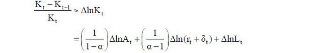
Thus, the change in the aggregate capital is attributed to the changes in TFP growth, changes in the components including the effects of changes in the factor prices, and changes in aggregate labor. Table 4 presents the decomposition of the growth rate of capital stock.
From about 3.1% per annum in the 2010s, the growth rate of capital demand is projected to be nearly 2.2% per annum in the 2020s and to decline further to 1.3% per annum by the 2050s. After 2020, the low growth of capital demand is attributable to the decrease in aggregate labor, because a gradual slowdown in TFP growth is assumed. Therefore, the demographic transition also contributes to the low GDP growth rate through the channel of capital accumulation by about −0.4% per annum in our baseline projection.9
In sum, the rapid demographic transition of Korea will place significant pressure on the GDP growth rate in the coming decades. First, the volume of aggregate labor supply is expected to shrink rapidly. Although the model economy includes a channel through which the female labor supply plays a greater role in the aggregate supply by a reasonable magnitude, the baseline projection shows that it is not enough to cancel the negative effects from the decrease in the working-age population, partly because the female population is also rapidly aging. Second, the decrease in the working-age population indirectly affects the GDP growth through the capital accumulation channel, as the decrease in the aggregate labor supply lowers the marginal productivity of capital.
V. Counterfactual Exercises
In the previous section, we examined the endogenous responses of the macro variables to the baseline projection assumptions. In this section, we separately examine the effects of exogenous variations in the decline in fertility, the increased life expectancy rate, and our assumption about the increase in female productivity.
A. Decline in Fertility and Increased Life Expectancy Rate
Our baseline projection indicates that Korea’s demographic transition is projected to have a significant effect on the Korean economy for a considerable period of time in terms of the GDP growth rate. The demographic transition is progressing in two ways: a decline of the net fertility rate and increased survival probabilities, especially for the elderly population. The first lowers the aggregate labor supply, as does the demand for investment in the long- run. However, the second factor may have a positive effect on the economy with regard to the growth potential. The rise in survival probabilities is equivalent to prolonged life-expectancy such that the incentives to work and save before retirement increase, resulting in an increase in the aggregate labor supply and capital accumulation. In this subsection, we conduct counterfactual simulations to quantify these effects separately.
The first scenario (S1) sets the net fertility rate to zero % in the year 1991 and assumes that it will stay at that level indefinitely. We then calculate the new equilibrium path of this economy with other parameters held constant.10 Table 5 presents the long-term GDP growth path under S1. Also shown in the parentheses is the baseline projection presented in the previous section. According to Statistics Korea, 686,000 children were born in 1991, but the number decreased to 449,000 in 2010. This declining trend is projected to continue, and 288,000 children are expected to be born in 2060. However, the difference in the number of children born in the 1990s is mostly negligible between the scenarios and noticeable differences in the model simulation appear in the 2020s. The absolute numbers of newborn children for both scenarios are shown in Figure 8.
In terms of the output growth rate, starting from the nearly identical results up to the 2000s, the gap starts to widen, on average, to 1.3%p per annum in the 2050s. The contribution of labor is projected to be 0.9%p higher and that of capital 0.4%p higher in the 2050s. In the model economy, people born in the 2000s, for example, start working in the 2020s and stay in the labor market for 45 years. Therefore, the effect of the very low fertility rate starts to become visible very slowly, but its cumulative effect is astounding. Under S1, as percentage deviations from the baseline simulation in the same year, the aggregate labor supply is 4.8% higher and the level of output is 4.4% higher in 2030. These numbers will continue to increase to 43.8% and 40.1%, respectively, by 2060.
According to Statistics Korea, life expectancy was 71.7 years in 1991 and 80.8 years in 2010. It is projected to reach 88.6 years by 2060. In order to quantify the effects of the increased life expectancy rate, the second scenario (S2) assumes that the survival probabilities do not improve after 1991 such life expectancy is fixed at 71.7 years. Table 6 presents the long-term output growth path under S2. Also shown in the parentheses is the baseline projection presented in the previous section. Compared to the baseline projection, capital accumulation is slower because there is less of a need to save for retirement. A shorter life expectancy rate also encourages households to enjoy more leisure during the working years; thus the aggregate labor growth is relatively slow compared to the baseline simulation. For these reasons, the output growth rate is lower by approximately 0.1~0.2%p per annum under S2. Under S2, as percentage deviations from the baseline simulation in the same year, the aggregate labor supply is smaller by 5.9% and the level of output lower by 6.2% in 2030. By 2060, the aggregate labor supply will be 7.9% below the baseline value and output 8.2% below the baseline value. Therefore, the effects of the increased life expectancy rate on the GDP growth rate partially offset the negative effects of Korea’s low fertility rate, although this is limited.
Despite the fact that it is not specified in our model economy, there are other channels through which the rise in life expectancy affects output growth positively. For instance, the rise in life expectancy is closely related to the improvement in the health status of the elderly population. If the working period over the life cycle increase as people live longer, so does the incentive to acquire human capital in the early period of the life-cycle. The effect of additional human capital accumulation on output growth may be greater if the accumulation of human capital could spill over into the economy. Of course, it is difficult to quantify the growth effect through the human capital channel.
B. Female Labor Supply
The discussions thus far indicate that the decrease in the aggregate labor supply due to the persistently low fertility rate will be a major factor behind the low growth potential of the Korean economy in the coming decades. As the size of the labor force shrinks, the female labor supply will increase due to market forces given the scarcity of labor. In addition, because Korea’s female labor participation rate is among the lowest all OECD member countries, as shown in Figure 9, there is sufficient room for improvement regarding the female labor supply.
FIGURE 9.
FEMALE LABOR MARKET PARTICIPATION RATE
Note: The labor market participation rate for working-age (15-64) females. The values are average values for 2010~2014.
Source: OECD. Stat.
Although our model does not have an explicit structure in which female workers choose whether to work or not, the baseline projection takes into account that the female labor will play a greater role in the future for with regard to aggregate labor supply. We assume that the age-productivity profile of female workers will increase and converge to that of male workers. In our model economy under the baseline scenario, the proportion of the female labor supply, in terms of the efficiency unit, will increase from 36% in 2013 to 47% in 2060. According to the Economically Active Population Survey, female workers took up approximately 42% of the total employment in 2013. Shin et al. (2013) reported that the proportion is projected to increase to 46% in 2060. Although these numbers are not directly comparable to the female labor supply in our model, we consider that our assumption regarding the role of the female labor supply in the future is somewhat optimistic as compared to that in Shin et al. (2013).
In order to quantify the consequences of our assumption, we conduct another simulation exercise in which we assume that the female age-productivity profile does not change after 2013. These results are reported in Table 7. Compared to the benchmark economy, the output growth rate is about 0.3%p lower in the upcoming decades because the contributions of labor and capital decrease by 0.2%p and 0.1%p, respectively. Under the alternative scenario, as percentage deviations from the baseline scenario in the same year, the aggregate labor supply is 13.8% smaller and the level of output is 10.8% lower in 2060. Moreover, when convergence in age-productivity is achieved, the output growth effect will vanish. For example, if we assume that female labor productivity increases twice as quickly relative to the baseline scenario, the level of output is only 0.9% greater than the baseline economy in 2060 and the difference converges to zero thereafter. However, output growth is faster during the period in which the female labor productivity increases.
Thus, we have concentrated on analyzing the implications of exogenous projection assumptions by deviating from the baseline scenario by considering the persistent low fertility (S1), improvement in life expectancy (S2), and the increase in female labor productivity (S3) in sequence. In order to gauge the relative importance of these assumptions for the baseline simulation in the long run and to view the results from a somewhat different angle, we conduct additional exercises.
We begin with a counterfactual exercise in which the growth rate of the new born population remains at zero percent after 1991, the survival probabilities do not improve after 1991, and the female age-productivity does not change after 2013. We refer to this set of model assumptions to as scenario M1. Starting with M1, scenario M2 replaces the zero new born population growth assumption with the baseline fertility assumption. To construct scenario M3, we add the longer life expectancy assumption to M2. Note that M2 coincides with S3. Lastly, scenario M4 is determined by adding the increase in the female labor productivity assumption to M3, which results in a set of assumptions identical to that of our baseline projection scenario. These results are reported in Table 8, in which all values are reported as percentage deviations from M1 in 2060.
TABLE 8
THE EFFECTS OF PROJECTION ASSUMPTIONS ON THE MACROECONOMIC VARIABLES
Note: All variables are reported as percentage deviations from M1 in the year 2060.
M1: No change
M2: No change + Low Fertility
M3: No change + Low Fertility + Life-expectancy
M4: No change + Low Fertility + Life-expectancy + Female Productivity
This sequence of exercises shows that the macroeconomic effects of Korea’s demographic transition are highly significant. Regarding output growth, the decrease in the working age population due to low fertility will pose a serious problem; as percentage deviations from M1 in 2060, the aggregate labor supply, capital stock, and output level are lower by 32.8%, 28.1% and 30.7%, respectively in 2060 under M2. Despite the fact that a longer life expectancy rate encourages economic agents to work and save more, the magnitude of the effect is limited; as percentage deviations from M1 in 2060, the aggregate labor supply, capital stock, and output level are correspondingly 26.9%, 21.7% and 24.9% lower in 2060 under M2. In addition, the increase in the female labor supply may partially offset the negative effects of the demographic transition; under M3, the aggregate labor supply, capital stock, and output level are likewise 15.2%, 16.3% and 15.6% lower than M1.
VI. Summary and Conclusion
The demographic change in Korea is expected to be rapid and drastic, at least for the next few decades. In this paper, we build an overlapping generation general equilibrium model to analyze the effects of the demographic changes on the GDP growth potential up to 2060. Under the assumption that the slowdown in the TFP growth rate will be only moderate in the future, remaining at 1.3% per annum, the growth rate of the Korean economy is projected to slow to 1.1% per annum in 2050s from 4.0% in 2000s. The shrinking workforce due to the decline in the fertility rate will play a significant role in the slowdown of the Korean economy. Moreover, although the increased life expectancy rate is expected to mitigate the negative effect, the magnitude of its effect turns out to be limited.
Our model is reasonably successful in reproducing the historical path of major macro variables, but there are also limitations. First, the government sector is not specified. In future research, the model economy could be extended to investigate the implications of aging in Korea on the public pension system and fiscal policies. Second, we are silent on the determinants of the future growth of TFP. We simply assume that it is exogenous and will grow at a predetermined rate. However, its contribution to output growth is becoming more important. To analyze the effects of the demographic transition on output growth fully, we must investigate the validity of this exogeneity assumption. This is not an easy task, but it is of importance especially for Korea, which is aging at an unprecedented speed.
Appendices
If a household of age j in period t exits from the economy, it leaves its assets, (1 + rt )a'(j − 1, t − 1), as an unintended bequest. We assume that the assets are distributed to its adult children’s generation. If it has no adult children, it is distributed to all living households equally.
Let si,j,t be the proportion of age-i adult children to all of the children born to the household of age j in period t. Then, we obtain si,j,t by
 if j − 20 ≥ 21
Let si,j,t denote the amount of assets that a household of age i in period t receives from a household of age j in period t. Then,
bsi,j,t = si,j,t (1 + rt)a'(j − 1,t − 1) if j − 20 ≥ 21
Therefore, the amount of assets the household of age j inherits in period t from its parent generation is
where the second term donates the amount of assets distributed equally to all living households.
Notes
In this paper, by output growth rate, we mean not the per capita output growth rate but the total output growth rate.
Therefore, the working-age population of the model economy consists of the population aged 21~64, which is different from the conventional definition of the working-age population (15~64).
See the appendix for details on the construction of bj,t. We assume that unintended bequests from a specific cohort are distributed proportionally to its children generations, unlike the standard equal distribution assumption. However, simulation results show no meaningful differences
In the same manner, the supply of aggregate capital in period t,  is equal to the total amount saved by the representative households in period t-1.
The two concepts are interchangeable under the assumption that the firm is under the constant returns to scale Cobb-Douglas production function and that the markets are competitive.
In the growth accounting by Cho (2014), labor input is measured as employment. However, it turns out that the trend in the TFP growth rates is very similar to that of Cho (2014). Therefore, we adopted their assumptions regarding the future TFP growth rate.
A close empirical counterpart of our aggregate labor can be constructed by total working hours weighted by the age-productivity profile. However, the time series of the average working hours can be obtained for the years after 2004, which is much shorter that the in-sample time horizon.
The contribution of capital in Table 2 is calculated as the growth rate of capital stock × the capital share (0.39).
References
, , & . (2007). Global Demographic Trends and Social Security Reform. Journal of Monetary Economics, 54(1), 144-198, https://doi.org/10.1016/j.jmoneco.2006.12.010.
, , & (2009). The Saving Rate In Japan: Why It Has Fallen And Why It Will Remain Low. International Economic Review, 50(1), 291-321, https://doi.org/10.1111/j.1468-2354.2008.00531.x.
, , & (2007). The Japanese Saving Rate between 1960–2000: Productivity, Policy Changes, and Demographics. Economic Theory, 32, 87-104, https://doi.org/10.1007/s00199-006-0200-9.
(1993). The Cyclical and Secular Behaviour of the Labour Input: Comparing Efficiency Units and Hours Worked. Journal of Applied Econometrics, 8(1), 71-80, https://doi.org/10.1002/jae.3950080106.
, & . (2007). On the Consequences of Demographic Change for Rates of Returns to Capital, and the Distribution of Wealth and Welfare. Journal of Monetary Economics, 54, 49-87, https://doi.org/10.1016/j.jmoneco.2006.12.016.
OECD. OECD, OECD.stat, http://stats.oecd.org.