- P-ISSN 2586-2995
- E-ISSN 2586-4130

This paper examines the impact of introducing high-speed trains on consumer welfare, taking the ensuing changes in train schedules into account. Based on the estimated demand model for travel which incorporates consumer’s heterogeneous preferences for travel schedules into the standard discrete-choice model, I separately evaluate the impact from adding high-speed trains and that from changes in train schedules. The results indicate that consumers who travel between two cities connected by high-speed trains benefit from the introduction of high-speed trains, while some travelers whose choice set does not include high-speed trains face a reduced frequency of non-high-speed trains, resulting in significant losses.
Endogenous product characteristics, New product entry, Consumer surplus, High-speed train, Korea, KTX
L13, L92
Generally speaking, introducing an additional differentiated product into a market benefits consumers due to the increased number of alternatives if everything else, such as prices, remains the same. However, the effect on consumer welfare is not as simple if producers also change the characteristics of other products and the set of other products offered. This paper considers firms’ reactions to the introduction of new products, particularly in cases of altered product characteristics or altered sets of products offered, and analyzes the effects of new products on consumer surplus, taking those reactions into account. The goal of this analysis is to investigate changes in consumer welfare due to the introduction of a new product based on available Korean transportation industry data. Specifically, this paper decomposes the effects of the introduction of high-speed trains into the gains or losses attributable to having high-speed trains and those attributable to firms’ choices of products to offer across different types of consumers.
This paper contributes to the literature by examining the effects of new product introduction considering firms’ choices of product characteristics in response to the new product. The possible effects of new product introduction can be explored by reviewing the considerable amount of literature available (Trajtenberg 1989; Petrin 2002).1 However, many of the empirical studies of markets with differentiated products primarily address firms’ pricing strategies given the characteristics of each product while treating the market structure as exogenous. Moreover, the effects of ensuing changes in product characteristics and the product line after the introduction of a new product have not been discussed substantially in the empirical literature despite the fact that corresponding theories are well documented (Spence 1976; Gabszewicz et al. 1986).2 Berry et al. (2006) and Berry and Jia (2010) also emphasize that producers may have an incentive to manipulate product characteristics other than prices.3 In particular, a rail company in Korea may have a strong incentive to control product characteristics such as train schedules, particularly because with regulation, it has only limited power over pricing. Accordingly, I will treat the choices of train schedules of the rail company as endogenous in all subsequent discussions, and I will account for this by using the instrumental variables in the estimation.
To study the effects of both new product introduction and the ensuing changes in product characteristics on consumer welfare, I estimate consumer demand for travel while explicitly incorporating preference heterogeneity into an otherwise standard discrete-choice model (Koppelman 2006; Train 2009). Heterogeneity is captured in my model through a modification of the concept of the “schedule delay,” the difference between a traveler’s most preferred time to travel and his or her actual time to travel, suggested in Miller (1972) and Douglas and Miller (1974). Although preference over the travel schedule is an essential factor with regard to travel demand, there has been limited modeling of it in the past due to data constraints. Some research that analyzes travel demand, such as that by Koppelman et al. (2008), models departure time preferences, but in general they consider neither potential endogeneity from the schedules nor the heterogeneity of preferences over travel schedules across consumers.
In my subsequent welfare analysis, I separately quantify the gains resulting from the introduction of high-speed trains and the welfare changes resulting from the rail company’s schedule adjustments. For the welfare analysis, I utilize the observed set of products offered in the Korean transportation markets before high-speed trains were introduced instead of estimating a model of supply owing to data limitations and ambiguity regarding the objectives of the rail company.
As a result of this research, I found that the introduction of high-speed trains caused sizable increases in consumer surplus in the Korean transportation markets where high-speed trains have been made available. However, due to the losses caused by the changes in the sets of products offered to consumers, the overall change in consumer surplus in the transportation market as a whole after the introduction of high-speed trains is smaller than the increases which resulted from the addition of high-speed trains. I also found that there are significant differences in the magnitude of consumer welfare changes across heterogeneous consumers. The benefits from the new product introduction are somewhat confined to a small number of markets, while the changes in choice sets affect a broader range of consumers.
The differential effects across consumers depend on the availability of high-speed trains. On the surface, consumers who had high-speed trains added to their choice set benefited as a result. However, this group of consumers endured approximately 50% fewer non-high-speed trains after the introduction, which offset the gains from the high-speed trains. Thus, the net gains for that consumer group are not as large as intuitively expected, as the schedule changes caused substantial welfare losses which offset 50% of the gains from having high-speed trains. Consumers who travel between two cities that are not connected by high-speed trains but are located along a high-speed rail line are also subjected to nearly 50% fewer trains owing to the reduced frequency of trains. As a result, that consumer group experienced only a loss in consumer surplus. On the other hand, consumers who travel between two cities which are not located along a high-speed rail line experienced an increased number of trains due to the reallocated conventional trains; thus, they experienced a substantially increased consumer surplus. These changes in train schedules are more noticeable than mere price changes after the introduction of high-speed trains, yielding more significant effects on consumer surplus than those of price changes.
The remainder of this paper is organized as follows: Section II explains the transportation industry in South Korea, and Section III presents the model. Section IV and Section V describe the data used and the estimation procedure and assumptions imposed, respectively. Section VI addresses the procedure used to calculate consumer welfare, and this is followed by a discussion of the results in Section VII. The summary and concluding remarks are offered in Section VIII.
Rail service in South Korea is provided by only one company, Korail, which leases railroads from the Korea Rail Network Authority. It currently operates four different types of trains, categorized in terms of speed: KTX, Sae-ma-eul, Mu-gung-hwa and Tong-il. It had been operating the latter three types prior to the introduction of high-speed trains in April of 2004. KTX, the high-speed train introduced in 2004, is the fastest train type available in Korea, making only a few stops during its trips. Sae-ma-eul is the second fastest train type. It skips small stations, but it stops at a large city in each region. Mu-gung-hwa can be regarded as a local train, stopping even at stations in small cities. In the analysis, only three types of trains are considered because Tong-il covers relatively short distances and is usually used by commuters who live in suburbs that are not reached by subways.
Korail was a governmental organization until 2004, at which time it became a public enterprise financed by the government. Although it became a corporation, its general behavior, such as its pricing strategy, did not change because the government is the only shareholder. It has extremely limited power regarding its pricing. In particular, the fares must only depend on the train type and the traveled distance, and the firm cannot set prices differently for a given destination within the same day. Specifically, Korail determines a “minimum fare” and a “rate per km” for each type of train subject to the maximum rate per kilometer announced by the Ministry of Land, Infrastructure and Transport and approval from the ministry, and calculates fares based on a combination of the train type and distance using what are known as “distance scale rates.”4 Similar to pricing, Korail must also obtain approval from the Ministry of Land, Infrastructure and Transport in order to change its service frequency. However, it has a degree of flexibility regarding its schedule frequency. Whereas Korail must earn the approval to change its frequency for each rail line by more than 10% according to the enforcement decree of the Railroad Enterprise Act, reducing the schedule by less than 10% and changing the composition of train types do not require approval.5
This paper takes advantage of these strict regulations on pricing. In the empirical literature, one major econometric issue is potential endogeneity bias caused by prices. That problem does not arise in this paper, as rail pricing is strictly regulated; therefore, prices are assumed to be uncorrelated with unobserved product characteristics. In addition, because the rail fare is identical for a given destination on the same day regardless of the departure time, consumers’ observed choices of travel schedule, such as “morning” or “evening,” reflect their preferences based solely on schedule without being influenced by price.
Although this paper focuses on the rail industry, it is still important to understand other modes of transit in order to analyze the demand for rail service. In particular, substitution between rail services and other modes of transportation influences the overall effect of the introduction of high-speed trains on consumer surplus. Therefore, it is important to take the market size and outside alternatives into consideration. I define outside alternatives here as traveling by bus, airline or car as well as foregoing travel.6 There are multiple bus companies operating on each route, and their pricing regulations resemble those of the rail company. Bus fares are calculated using “Distance Scale Rates,” and fare changes are similarly subject to governmental approval. There are two major airline and three low-cost carriers. Routes between the mainland and Jeju Island are excluded because rail service does not compete with airlines in these routes. Air fare pricing is much less restrictive than that of rail fares. Fares can be set at the discretion of airline companies as long as they provide public notice in advance. Changes in air fares are rarely observed, however.
In order to evaluate consumer surpluses resulting from the introduction of high-speed trains, one must analyze the demand that describes how travelers choose a means of transportation, taking into account their preferred travel schedules. I estimated the demand for travel using a discrete-choice model used effectively in the past. (See Berry 1994; Berry et al. 2006; Koppelman et al. 2008; Berry and Jia 2010; Ho 2006) I also extended the standard multinomial logit model by allowing for heterogeneous travel schedules among consumers.
This section describes in detail markets and products as I have conceptualized them in this research.
A “market,” as used in this paper, is defined as unidirectional travel from an origin city to a destination city. Each unique market is identified by a unidirectional city pair and a month. Each market has its own set of products offered. A “product” is defined as a specific train operating on a specific route (a unidirectional pair of two stations) within a specific market. Each train, which is identified by a unique ID number, runs from a start-node station to an end-node station, with additional stops made during the trip. This definition of a product therefore implies that a single train connecting cities A, B and C is treated as a different product for the two connections it makes (A to B and B to C) because it operates on two distinct routes. Furthermore, given that each city may have more than one station, multiple routes can exist. Therefore, even within a given market, consumers face product choices depending on route preferences. This implies that a train running route 1 (station A1 in City 1 to station A2 in City 2) and the same train running route 2 (station B1 in City 1 to station B2 in City 2) are treated as different products even if both trains have the same train ID number and both routes are engaged in the same market.
In reality, travelers can transfer from one train to another or change modes of transportation over the course of a single trip. However, my analysis could not reflect travelers’ transfer decisions throughout the itinerary because the dataset provided by Korail does not contain information regarding individual passengers’ itineraries; therefore, that data could not support a trip-based analysis. I attempt to work around this problem, at least partially, by defining a product as a combination of a route and a train ID rather than as the complete trip an individual traveler conceptualizes. A single rail trip is therefore a series of products, as defined above, in that a traveler may take different trains for each section of his trip.7 A traveler who wants to travel from A to C with a transfer at B chooses a product for A-B and another product for B-C. Although the traveler is one person, he or she will be treated as two separate travelers in the model because a city pair from A to B and a pair from B to C are two different markets.
The characteristics of each product are inherited from the respective product’s train and that train’s routing. The characteristics of a train are its type, fare, traveled distance, and schedule. The characteristics of a train’s routing include the distance from the station to the city center and the number of trains scheduled for the route within a day. Those characteristics of a train’s routing attempt to explain the convenience of each route in terms of intra-city transportation.
This paper attempts explicitly to incorporate traveler’s heterogeneous travel schedule preferences. Because the fares for a given product do not vary on the same day, I assumed that travelers’ schedule choices are based entirely on the schedule themselves. This ignores the fact, however, that travelers may need to travel at times other than those they prefer due to train availability.8 Personal preference is compromised even more if a traveler wants to take a specific type of train because it decreases the likelihood of traveling at a preferred time even further. Thus, the difference between travelers’ most preferred travel times and the actual times chosen could cause inconvenience, and this can significantly affect the demand for trains. In order to measure this potential traveler inconvenience, I adopted the notion of schedule delay from Douglas and Miller (1974) and Miller (1972), which define it as the absolute difference between the passenger’s most preferred time to travel on 24-hour clock and that of his actual time to travel. Each traveler’s schedule delay causes disutility.9
This paper assumes that each traveler has a target time in mind for one endpoint of each potential trip that does not vary with mode or schedule choices. In existing literature that discusses preferences over travel schedule, departure time is usually considered instead of arrival time (Douglas and Miller 1974; Koppelman et al. 2008). Although it is not common to use preferences over arrival time, this paper adopts arrival time for the travel schedule because a traveler normally chooses a departure time and a mode of transportation with a target arrival time in mind. His preferred departure time therefore depends on how he travels, while his target arrival time remains constant during the selection process. In this context, using preference over arrival time instead of departure time is more consistent.10
The logit model with traveler’s heterogeneous preferences with respect to travel time will be adopted in this paper. A traveler i, whose preferred travel time is hi, faces a choice problem over products given a city pair m during time period t: he has to choose how to travel.11 Traveler i will consider all of the products in the market mt to choose a product that yields the highest utility. This paper assumes a linear utility (or disutility); hence, the utility function of traveler i for product j (a train-route combination) is given by
where vector xj. contains the observed characteristics of each product, including the fare. Because the heterogeneity of city pairs is very large, the model includes a dummy variable for each city pair m - the coefficient on the dummy variable for city pair m is ηm - in the demand to allow for the valuation of inside goods to differ across markets. γ·d(ajmt, hi) measures the inconvenience caused by a schedule delay, where γ<0. d(ajmt, hi) is the absolute difference between ajmt and hi, hi is traveler i’s preferred travel time of day, and ajmt is his actual time of day to travel specifically on product j in market mt.12
The product-level unobservable ξjmt accounts for a number of product characteristics which are not observed by econometricians,
such as the unobserved characteristics of the routes or trains, the facilities inside
each train or in the train stations, and the quality of the train attendants.  is an additive error term, specific to product j in market mt, which is assumed to follow an extreme value distribution and to be distributed independently
across both consumers and products.13,14 This error term captures each traveler’s idiosyncratic tastes with regard to trains
or routes, or possibly his physical location or the purpose of his trip.15
is an additive error term, specific to product j in market mt, which is assumed to follow an extreme value distribution and to be distributed independently
across both consumers and products.13,14 This error term captures each traveler’s idiosyncratic tastes with regard to trains
or routes, or possibly his physical location or the purpose of his trip.15
I explicitly introduced “outside” alternatives in Section IV, which include traveling by modes of transportation other than trains as well as not traveling. The mean of this utility from the outside alternative is normalized to be zero. The coefficients of city-pair-specific dummy variables (ηm) in the utility of “inside goods” are interpreted as being relative to the outside goods.
Given the utility function (1), each traveler i purchases one unit of a product j that yields the highest utility. That is, conditional on (xmt, ηm, ξjmt, amt) and his preferred time to travel hi, he will purchase one unit of j if and only if  ∀k∈Jmt∪{0}, k≠j, where Jmt is the set of products available in market mt and {0} is the set of outside alternatives.
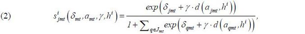
The market share of a product is defined as the percentage of travelers using that product out of all potential passengers. The market size is discussed in Section IV. Based on the assumption of the distribution of ϵ, the probability that traveler i purchases product j conditional on (xmt, ηm,ξjmt, amt) and i’s preferred time to travel is given by the well-known formula
where δjmt=xjmtβ+ηm+ξjmt, and which is shared among all travelers in the market.
If the distribution of hi is known, the market share for each product can easily be obtained from the expectation of (2) over hi. This paper assumes the traveler’s preferred time of day to travel to be discrete such that each traveler has his preferred “hour” to travel on a 24-hour clock. This allows the model to be a discrete mixture of logit models. In other words, hi takes an integer between 1 and 24,16 and its probability mass function is Prob(hi=τ) = ϕτmt ∀τ∈B, where B is the set of support of hi, the 24 integers between 1 and 24. The overall market share of product j is
where ϕτmt denotes the percentage of travelers out of all potential travelers in market mt whose preferred time to travel is τ.
Although this paper does not contain any random coefficient, the model is similar to the mixture model with random coefficients due to the existence of hi. Ideally, the variable ϕτ, defined as the proportion of travelers whose preferred time is τ, can be estimated from the model; however, it is not practical to estimate a different vector of ϕ for each market. Such a task would be impractical even if it was assumed that the distribution travelers is common across markets, as estimation is difficult and is sensitive to small changes in the specification or instruments, as noted by Berry and Jia (2010).17
To sidestep this issue, this paper uses a proxy for the proportion of potential travelers
with preferred travel time τ, as obtained using the following assumptions. First, I assumed that the distribution
of travelers’ preferred times to travel varies across city pairs but does not vary
across time periods. That is, 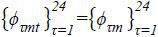 , ∀t. I also assume that the distribution of hi is identical across all alternatives. Let wτm be a proxy for the proportion of travelers in city pair m whose preferred time to travel is τ. Replacing ϕτmt with the proxy wτm allows the overall market share for product j to be rewritten as
Next, it is essential to find a proxy for  for each m which reflects the distribution of travelers’ preferred times of day to travel. The
process of constructing the proxy is based on the underlying belief that all travelers
will travel at times that are close to their most preferred times. This is a plausible
assumption because fares do not vary on the same day. Therefore, the preference for
a given travel time can be inferred by the number of travelers during that time. Thus,
one reasonable candidate for the distribution of hi is the hourly train ridership in each market as sourced from historical data. This
assumes that the company schedules trains to support travelers using their knowledge
of the true distribution of consumer preferences with regard to travel schedules;
thus, the hourly ridership should reflect travelers’ true preferences. I obtained
the proportion of travelers in each city pair m who actually travel during time period τ using
for each m which reflects the distribution of travelers’ preferred times of day to travel. The
process of constructing the proxy is based on the underlying belief that all travelers
will travel at times that are close to their most preferred times. This is a plausible
assumption because fares do not vary on the same day. Therefore, the preference for
a given travel time can be inferred by the number of travelers during that time. Thus,
one reasonable candidate for the distribution of hi is the hourly train ridership in each market as sourced from historical data. This
assumes that the company schedules trains to support travelers using their knowledge
of the true distribution of consumer preferences with regard to travel schedules;
thus, the hourly ridership should reflect travelers’ true preferences. I obtained
the proportion of travelers in each city pair m who actually travel during time period τ using
where  is the set of available trains in market mt with schedule τ,and qjmt is the number of passengers purchasing product j.18 I construct a proxy for
  for each m, smoothing the proportion of travelers in city pair m who actually travel at τ above the using Kernel density estimation.19
The main analysis employs three different sets of data. This dataset is self-constructed using raw data provided by Korail, the Korea Airports Corporation (KAC), the Korean Statistical Information Service (KOSIS) and the Statistical Yearbook of Land, Transport & Maritime Affairs. The first dataset pertains to the South Korean railroad industry and consists of market shares and product characteristics for the years 2006 and 2007. The second dataset includes the market size and the market share of outside alternatives. These two datasets, used in the demand estimation, only contain observations during the period after the introduction of high-speed trains. The third dataset contains the characteristics of products offered to travelers in 2002, when high-speed trains were not available. This dataset is used for the calculation of travelers’ surplus and the welfare analysis.
The first dataset pertaining to the railroad industry combines three different types of information from the Korean railroad (Korail) - i) the number of train passengers for each route (defined as a directional pair of stations) by train type and departure time of day aggregated monthly; ii) the major characteristics of each route, including fares, travel distances, and distance from a station to a city center; and iii) the train schedules with train types, routes, departure times and arrival times. In all, the dataset covers 6,456 routes throughout the country in existence during the time period of the data, and it contains the monthly aggregate numbers of train passengers for each route by train type and departure hour of day, observed for 12 months between July of 2006 and June of 2007. This dataset also contains the major characteristics of the route-train types of combinations, such as fares, travel distances, distance from a station to a city center, i.e., the key variables in the demand estimation.
The schedule data provides for each train identified by a train identification number, the stations at which stops are made, the train type, and the departure and arrival times. The ideal dataset for my research would include the numbers of train passengers aggregated for each train and for each route to facilitate more robust cross-referencing with the schedule of train services.20 Unfortunately, the available data only summarizes counts by train type and the hour of the departure time; therefore, to infer a train-level dataset, I imposed an assumption on the distribution of train passengers over trains departing within an hour. Each train for each route within a given hour is assumed to have the same number of passengers. Using this assumption, the unit of observation for the combined data is a single train, identified by its train identification (ID) number, running on a specific route over a month. Therefore, my analysis treats a train running on route A and a train running on route B as different observations even if the train ID number is identical.
The second dataset contains the market size and market share of the outside alternatives. “The market” as used herein is defined as a one-way travel choice from an origin to a destination city; hence, I treat a directional city pair and month combination as a separate market. “Travel choice” refers to traveling by rail, bus, car or domestic flight or choosing to forego travel. Potential travelers were estimated rather than observed, however, by assuming that the number of potential travelers is proportional to the geometric average of the populations of the two respective cities constituting a route (Berry et al. 2006).
Table 1 summarizes the data used in the demand estimation of this paper, which combines the first and the second datasets. It contains 392,459 products (station pair and train ID combinations) over 1,114 directional city pairs and 12 months. Therefore, the number of city pair and month combinations, which is recognized as a market, is 13,347. I excluded one of four train types, Tong-il, from the first dataset, because this type is usually used by commuters who live in suburbs which are not reached by subways, as discussed in Section II. Thus, it services a demand different from that focused on here. On average, 182 passengers travel on a train-route combination over the period of one month. N(Own Type Train/Day), N(Other Type Train/Day) and Station-City Centers are the variables used to capture the convenience of each route. N(Own Type Train/Day) counts a single type of train scheduled for a particular route within a day. N(Other Type Train/Day) similarly counts the other types of trains. The distance from the city center for a given route is defined as the sum of the distances between the departure and arrival stations from their respective city centers. This variable is meant to capture how conveniently located departure and arrival stations are in terms of intra-city transportation.
The price variations within a market primarily come from price differences across train types and from routings, as the fares for each route-train type of combination do not vary on the same day or between markets due to the distance-scaled rate system. Another source of price variation is nominal rail fare changes, which were observed twice in my data period. A third dataset is employed to compare travelers’ surplus before and after the introduction of high-speed trains. It contains information on the products offered to consumers before high-speed rail was inaugurated. Table 2 compares the number of products offered in 2006 with that in 2002 by train type. Each panel summarizes a specific type of train. The first row of each panel (N) shows the number of city pairs for which the given train type is available, and the next three rows show the mean, median and standard deviation. Each column of the panels summarizes a separate group of markets. In order to compare the train frequencies in 2006 to those of 2002, I partitioned markets into three groups based on high-speed train availability and location. Group 1, containing the city pairs with high-speed connections, is summarized in Columns (1) and (4). Group 2, containing the city pairs which are located along a high-speed rail line but are not connected by a high-speed train, is summarized in Columns (2) and (5). The city pairs that belong to Group 3, which are not on a high-speed rail line (and thus are not connected by high-speed trains), are summarized in Columns (3) and (6).
Note: 1) N: the number of city pairs in each group where each type of train is available. 2) Group 1: City pairs with a high-speed connection. 3) Group 2: City pairs on high-speed rail lines without available high-speed trains. 4) Group 3: City pairs that are not located along high-speed rail lines.
Each group has been affected differentially by the introduction of high-speed trains. The numbers of Mu-gung-hwa trains offered to Group 1 and Group 2 markets in 2006 were significantly lower than in 2002, while the numbers of Mu-gung-hwa trains offered to markets of Group 3 did not decrease substantially. The panel for Sae-ma-eul reveals two distinctive patterns. First, the numbers of Sae-ma-eul trains offered to Group 1 and Group 2 markets in 2006 also decreased compared to those in 2002.21 This change was caused by major reductions in the number of train scheduled for the routes along high-speed rail lines. Second, the panel also reveals that the number of city pairs where Sae-ma-eul trains are available increased from 127 city pairs to 260. This increase occurred because Sae-ma-eul trains stop more frequently and therefore became available in the cities where these additional stops are made. Group 3 experienced only relatively minor changes. In that group, Mu-gung-hwa trains became available between more city pairs despite the average number of Mu-gung-hwa trains slightly decreasing in the group of markets. The average number of Sae-ma-eul trains increased slightly for Group 3.
To estimate the demand parameters (β,γ), I followed the standard procedure proposed in Berry et al. (1995) due to the presence of the unobserved product characteristics ξ , and due to the presence of the heterogeneous travel time preference hi.22 Therefore, I inverted the following market share equation for each market to solve for the vector of δmt as a function of the data and the parameters to be estimated,
where smt(δmt,amt,γ) is a vector of the market shares in market mt, as described in (3), and  is a vector of the observed market shares in market mt. As in Berry et al. (1995), this system of equations is nonlinear with regard to the parameters to be estimated;
however, they can be solved numerically by means of contraction mapping.23 As described in Nevo (2000), I use two-stage least squares, which solve the linear parameters β as a function of the nonlinear parameter γ and limits the nonlinear search in the generalized method of moments to the nonlinear
parameter only.
is a vector of the observed market shares in market mt. As in Berry et al. (1995), this system of equations is nonlinear with regard to the parameters to be estimated;
however, they can be solved numerically by means of contraction mapping.23 As described in Nevo (2000), I use two-stage least squares, which solve the linear parameters β as a function of the nonlinear parameter γ and limits the nonlinear search in the generalized method of moments to the nonlinear
parameter only.
With this assumption, the rail company considers travelers’ schedule preferences when determining train schedules; therefore, E(ξmt) could be non-zero. Accordingly, we must include a set of exogenous instrumental variables to identify the parameters. The moment conditions used in the estimation are derived from E(ξmt | zmt) = 0 , where zmt is a vector of instruments. For any vector of function h(·), the moment conditions imply E(ξmt · h(zmt)) = 0. 24
Although strict regulations on pricing mitigate the endogeneity problem from prices, the endogeneity from train schedules is of concern in this research. Because a rail company in Korea has only limited power over pricing, it may have a strong incentive to control product characteristics, such as train schedules, instead of fares. As a result, the arrival time of product j, amt and the schedule delay, d(ajmt,hi) may be endogenously determined by the rail company.25 Therefore, it is necessary to include valid instruments in order to identify the demand model.
The identification strategy used in this paper searches for the variables that affect the rail company’s schedule decisions, but not those that affect consumer demand, exploiting the special circumstances of the railroad industry. Consider, for example, trains running along rail line A with stops at stations between A0 through AN+1 (N intermediate stations). When a rail company determines the schedule for those trains, it would ideally consider the levels of demand for each of the individual routes along the railroad. However, a traveler would care only about the routes on the market in which he travels.26
The demand estimates provide information about how consumers value each of the product characteristics. These results indicate that consumers experience significant disutility from traveling at a time other than their preferred time to travel. The next step is to quantify the changes in consumer surplus after the introduction of high-speed trains. Because the train schedules changed as a result of the introduction of high-speed trains, I separately considered the changes in consumer surplus caused by train rescheduling and those caused by the introduction of high-speed trains.
The change in consumer welfare can be measured according to the difference between the expected utilities in two different situations. I primarily compared consumers’ expected utilities from the set of products offered after the introduction of high-speed trains to those from the products offered before high-speed trains were introduced. To examine the effects of the introduction of high-speed trains separately from other changes, such as train reallocations, I considered consumer surplus with six different sets of products, followed by a stepwise comparison to illustrate the effects of situation changes. It is important to note that the expected utility calculation is based on the observed sets of products and not based on the optimal scheduling choice of the rail company from a supply-side model. The six product sets are defined as follows:
(S1) Train schedules offered to travelers in 2002, before high-speed trains were available, using the prices from 2002
(S2) Train schedules offered in 2002, before high-speed trains were available, using the prices from 200627
(S3) High-speed train schedules offered in 2006, including the other types of trains considered in (S2), using the prices from 2006
(S4) Identical to the product set in (S3), but excluding trains that were no longer part of the 2006 schedule, using the prices from 2006
(S5) Identical to the product set in (S4), but including trains that were newly offered in 2006 versus 2002, using the prices from 2006
(S6) Train schedules offered in 2006, using the prices from 2006
(S1) and (S6) present actual situations, whereas the others present hypothetical situations. The changes from (S1) to (S2) correspond to the effects of price changes between 2002 and 2006. A comparison between (S2) and (S3) provides the effects of the introduction of high-speed trains on travelers’ surplus. The changes from (S3) to (S6) corresponds the effects of schedule changes after the introduction of high-speed trains, and the stepwise comparisons from (S3) to (S6) break down those effects into three components: the effects from the elimination of trains ((S3)→(S4)), the effects from the addition of trains ((S4)→(S5)), and the effects from the pure reallocation of existing trains ((S5)→(S6)).
To break down the effect of schedule changes into the three components discussed above, it is necessary to group the trains offered in 2002 into those subsequently removed in 2006 and those still remaining in 2006. Because the systems used to assign identification numbers to trains were different in 2002 and 2006, it was not possible to use the train identification number for the sorting. Thus, this paper exploits the partition of hours, which is defined in Section III.C, by matching Morning trains offered in 2002 to Morning trains offered in 2006 based on the arrival time and the train type. For example, if there were five Mu-gung-hwa trains in the Morning group in 2002 and there were six Mu-gung-hwa trains in the Morning group in 2006, I paired the first offered in 2006 with the five trains offered in 2002 and considered them as trains with “adjusted schedules.” The single remaining train was then considered as “an added train.” Under this sorting rule, a change in the schedule of a train within time group (Bg) was considered as a reallocation, whereas scheduling a train such that it fell into a different time group (Bg', g'≠g) was considered as a removal of that train from the first time group (Bg) and the addition of a new train to the second time group (Bg'). Using a different sorting rule could result in a different distribution of consumer welfare changes across “removing trains,” “adding trains” and “reallocating trains;” however, the total effects of “schedule changes,” which consists of all three changes, is invariant across different sorting rules.
To approximate the expected utility given the estimated demand, this paper replaces
ϕτmt, the proportion of travelers whose preferred time to travel is τ, with the proxy wτmt, as defined in (5). Because in (1) is assumed to have an extreme value distribution, the expected utility can
be rewritten as
and a monetary measure of the change in travelers’ welfare, EVmt, can be constructed according to
where βp is the price coefficient and Mmt is the market size of mt (Ben-Akiva 1973; Nevo 2003).  and
and  represent the expected utilities of situations with high-speed trains and without
these trains, respectively; thus, (8) allows us to compare two different situations
with the same demand system.28
represent the expected utilities of situations with high-speed trains and without
these trains, respectively; thus, (8) allows us to compare two different situations
with the same demand system.28
Table 3 shows the results of demand estimations based on the main specification that takes both travelers and non-travelers into consideration. Table 3 shows the estimated parameters, which include the mean utility parameters (β) and the parameter representing the disutility from schedule delay (γ). Column (1) shows the parameters using the main specification, and Column (2) shows the same parameters estimated using the same model without employing the excluded instrumental variables. Column (3) shows the parameters resulting from an OLS estimation of δjmt.
Note: 1) N=392,459; N(Markets)=13,347; N(City Pairs)=1,114. 2) ***Significant at p=0.01; **Significant at p=0.05; *Significant at p=0.1
The mean estimated utility of high-speed trains (KTX) is higher than that of other types of trains for long-distance trips. To be specific, the mean utility values for the KTX are 0.37, 1.81, 3.07 and 4.15, while the mean utility values for Sae-ma-eul trains are 0.3, 0.92, 1.41 and 1.77 for 100 Km, 200 Km, 300 Km, and 400 Km trips, respectively.29 Schedule delay has a significantly negative impact on demand. In Column (1) of Table 3, the estimated coefficient for schedule delay is −0.311. The most straightforward method of interpreting this coefficient is to compare it to the price coefficient. The price coefficient (−0.115) and the coefficient for schedule delay imply that travelers are willing to pay as much as (approximately) 2700 KRW to reduce their schedule delays by one hour, holding everything else fixed. The coefficient for price shows that consumers are not sensitive to prices. To be more specific, the probability that they will purchase a product decreases by 9.9% when the price increases by 10%.
The examination of the estimated coefficients of the variables that indicate the convenience of each route, such as N(Own Type Train/Day), N(Other Type Train/Day) and Station-City Center, reveals that routes with more trains scheduled provide higher utility for travelers. In particular, N(Own Type Train/Day) and N(Other Type Train/Day) capture the frequency of the rail service for a given route, and more frequent service for a route implies that the route is more convenient than other routes in the market.30 The number of a given type of train scheduled on the same day affects a traveler’s utility more than the schedules of other types of trains. If the number of a given type of train scheduled on the same day increases by 10%, travelers choose corresponding products with a 7% higher probability. On the other hand, a 10% increase in the number of other types of trains scheduled on the same day results in only a 0.8% higher purchase probability. The distance between the station and city center is also an important factor affecting demand based on the estimated parameters. If a given station was relocated 10% farther from its city center, consumers would choose the corresponding products with a 9.5% lower probability.
I partitioned the markets into three groups based on high-speed train availability in the same manner used in Table 2. This partitioning facilitates an examination of the different effects across heterogeneous consumers. The results for Group 1, which considers consumers in markets with high-speed train stations, are shown in Column (1) of Tables 4, 5 and 6. Group 1 contains 107 million travelers per month across 107 city pairs. Column (2) of Tables 4, 5 and 6 summarize the results for Group 2, which consists of markets that are located along high-speed rail lines without available high-speed trains. Group 2 contains 190.7 million travelers per month across 330 city pairs. The consumers not accounted for in the first two groups belong to Group 3, whose results are shown in Column (3) of Tables 4, 5 and 6. Group 3 covers 615 city pairs with 348.9 million travelers per month. Consumers in Group 1 and Group 2 were expected to experience stronger effects from both the introduction of high-speed trains and the resulting schedule adjustments than consumers in Group 3. I summarized the changes in consumer surplus based on these groups. Tables 4, 5 and 6 reflect the main findings of this paper.
Note: 1) The result is based on the estimates shown in Column (1) in Table 3. 2) Group 1: City pairs with a high-speed connection. 3) Group 2: City pairs on high-speed rail lines without available high-speed trains. 4) Group 3: City pairs that are not located along high-speed rail lines.
Note: 1) The result is based on the estimates shown in Column (1) in Table 3. 2) Group 1: City pairs with a high-speed connection. 3) Group 2: City pairs on high-speed rail lines without available high-speed trains. 4) Group 3: City pairs that are not located along high-speed rail lines.
Note: 1) The result is based on the estimates shown in Column (1) in Table 3. 2) Group 1: City pairs with a high-speed connection. 2) Group 2: City pairs on high-speed rail lines without available high-speed trains. 3) Group 3: City pairs that are not located along high-speed rail lines.
Table 4 summarizes the expected consumer surplus changes per person for each market. Each subpanel in Table 4 displays the change in consumer welfare resulting from each of the five different sources described in Section VI. The “Price Change” panel shows the estimated change in consumer welfare due to price differences between 2002 and 2006. Given that rail fares decreased for 50% of the products available in my dataset, the changes in consumer surplus due to price change are positive. The “Add KTX” panel shows the gains which are attributable to the introduction of high-speed trains into the markets. Considering that high-speed trains became available in the markets of Group 1, only the consumers in Group 1 directly benefited from the new service. The next three subpanels summarize respectively the changes in consumer welfare due to the reduced number of scheduled trains, the scheduling of additional trains, and the rescheduling of existing trains to another time within the same day. The “Total Effect” panel reflects the overall changes in consumer surplus resulting from all sources having an impact.
Each column in Table 4 shows the heterogeneous impacts all normalized to be per person on consumers in each of the three groups, as described above.31 The median of the expected per-person change in Group 1 resulting from the introduction of high-speed trains is 5,600 KRW, but the expected change resulting from train schedule adjustments is −1,900 KRW, offsetting some of this gain.32 The median of the expected per-person loss in Group 2 resulting from schedule adjustments after the introduction of high-speed train is approximately 11,140 KRW. This loss occurred because some trains that were available before high-speed trains were introduced became unavailable after they were introduced. Group 3 consumers experienced only minor changes overall compared to consumers in other groups. The median of the expected per-person change in consumer welfare in Group resulting from schedule adjustments after the introduction of high-speed train is about 1,900 KRW. The total effect summarizes the changes in consumer welfare compared to that in 2002. The median of the expected consumer surplus change per person in Group 1 is 4,000 KRW, while that in Group 2 is −8,500 KRW.
Table 5 summarizes the expected consumer surplus changes in each market, taking into consideration market sizes and the magnitudes of the impact per person.33 The results obtained using the main specification demonstrate that both the introduction of high-speed trains and the ensuing changes in train schedules had substantial effects on consumer welfare, and that the size of the impact varied across consumers. The fact that the median and mean impacts are substantially different suggests that the changes in consumer surplus are heterogeneous across markets. Although the mean of the expected per-person consumer surplus change in Group 1 resulting from the reallocation of trains is positive, the mean calculated per market value is negative. This implies that the losses resulting from reallocating trains occurred in larger markets, which tended also to be more strongly affected by the introduction of high-speed trains directly, while some other markets in Group 1 benefited.
Table 6 summarizes the gross changes in consumer surplus in each of the three groups. As indicated earlier, rail fares decreased for 50% of the products available in my dataset; thus, the overall change in consumer surplus due to a price change was positive. The second row in each panel shows the gains stemming from the introduction of high-speed trains into the markets. In that high-speed trains became available in the markets of Group 1, only the consumers in Group 1 benefited from the new high-speed rail service. More concretely, the introduction of high-speed trains caused an estimated 10 trillion KRW increase in consumer surplus per month. The net gains for travelers in Group 1 are not as large as superficially anticipated, however, because schedule changes such as the reallocation and reduction of non-high-speed trains caused sizable losses that offset 50% of the direct gains resulting from the introduction of high-speed trains.
The next three rows (rows 3-5) summarize the changes in consumer welfare due to rescheduling trains, such as reducing the number of scheduled trains, scheduling additional trains and reallocating existing trains to another time slot on the same day. The consumer welfare change due to schedule adjustments in Group 1 markets was about −560 billion KRW. Consumers in Group 2 suffered a considerable amount of loss, −2.4 trillion KRW, due to changes in the set of products offered because train schedules in the corresponding markets were reduced by more than 50%. Without any added benefits from new high-speed services, consumers in the markets of Group 2 experienced losses three times higher than the gains of Group 1 resulting from the introduction of high-speed trains. On the other hand, consumer welfare in the markets of Group 3 increased by nearly 2 trillion KRW. Although some trains were removed from the original schedules, the gains resulting from additional non-high-speed trains and from reallocated trains outweighed the losses stemming from the removal of trains. Unlike consumers in Groups 2 and 3, consumers in Group 1 suffered a loss of 73 billion KRW resulting from trains being rescheduled to other time slots, as KTX trains are primarily scheduled at peak times and non-high-speed trains are primarily scheduled away from those times.
Overall, the gains from having high-speed trains are substantial. However, the losses from schedule adjustments that consumers were subjected to in the markets located along high-speed rail lines without high-speed trains scheduled outweighed those gains. Overall changes in consumer surplus were about 317 billion KRW; however, the positive changes are led by the gains from schedule adjustments in the Group 3 markets, but the gains from high-speed trains do not exceed the losses that occurred due to schedule reductions in Group 2 markets.
To summarize, introducing high-speed trains substantially raised consumer surplus in markets where they were actually made available. The changes in the set of products offered to consumers offset 50% of the gains, however. This resulted in greater losses of consumer surplus in markets located along high-speed rail lines but not connected by high-speed trains, and those losses outweighed the gains stemming directly from the introduction of high-speed trains. The overall change in consumer surplus after the introduction of high-speed trains was positive because the gains resulting from schedule adjustments in markets that are not located along high-speed rail lines made up for the losses in markets that are located along high-speed rail lines without available high-speed trains. I also found that there are substantial differences in the magnitudes of consumer welfare changes across heterogeneous consumers. The benefit gained directly from high-speed trains is concentrated in some of the markets, although changes in the choice sets affected a broader range of consumers.
A critical limitation of these results is an implicit assumption of the stability of the demand system. This approach presumes that consumers had identical levels of demand over product characteristics regardless of the existence of the new product. The results are derived based on the estimates of an indirect utility function for the period after the innovation despite the fact that the ex ante and ex post welfare calculations provide quantitatively different measures (Trajtenberg 1989). Given that the estimated demand is only based on the revealed preferences observed for the periods after the introduction, the calculated consumer surplus is valid only if the functional form of the demand is stable as we move away from the center of the data.
A more serious problem arises due to the distribution of travelers’ preferred times. First, we cannot guarantee that the distribution of travelers’ preferred times is time-invariant. The assumption imposed when the proxy for ϕ is constructed could lead to bias in the results. I used hourly train ridership in each market from the historical data for the proxy, assuming that the train schedule and hourly ridership reflect travelers’ true preferences. However, this could lead to a biased result if the preference with regard to travel schedule changed after the introduction because scheduling trains in a different way from that observed in 2006 will result in welfare losses. I believe that this bias is not serious because i) the welfare implication is robust under other distributions, and ii) the proportion of welfare changes due to schedule preferences is relatively small compared to those coming from schedule frequencies.
Lastly, the model adopted in this paper focuses on heterogeneous preferences for travel schedules rather than heterogeneous sensitivity levels to fares and schedule delays. However, in reality, sensitivity would affect a consumer’s modal choice together with sensitivity to prices.
In this paper, I addressed the effect on consumer surplus resulting from the introduction of high-speed trains and the ensuing changes in train schedules. I examined the impacts of introducing high-speed trains on consumer welfare using Korean transportation industry data, taking changes in the product selection offered by the rail company into account. With this data, I estimate a model of travel demand that incorporates consumers’ heterogeneous preferences for travel schedules into a standard discrete-choice model and compare the consumer surplus resulting from a set of products offered to consumers before and after the introduction of high-speed trains. My results show that the newly introduced highspeed trains had differential effects on consumers and that the ensuing changes in train schedules also indirectly affected consumer surplus. The changes in consumer surplus within a market depended on the availability of high-speed trains. The overall consumer surplus after the introduction of high-speed trains increased; however, the increase was not nearly as substantial as the gains directly resulting from the introduction of high-speed trains owing to the losses incurred by groups for which high-speed trains were not available.
My research calls attention to the impact on consumer welfare from cases of new product introduction and the subsequent changes due to the reactions of economic agents in related industries. Although the subsequent changes may have a substantial influence on consumer surplus, the scope of the investigation can easily be restricted to one specific industry or a particular group of consumers, and such a restricted scope can lead to biased results pertaining to welfare implications. This study also provokes a discussion regarding government spending. As expected, the construction of high-speed rail lines was costly and the Korean government allocated an enormous budget, which was levied from all taxpayers. However, the benefits tend to be concentrated in a few markets despite the diffused costs. Therefore, a thorough investigation regarding the benefits of government spending and its wider impact as well as an in-depth discussion are essential for better decisions regarding the government’s investments.
The numbers of airline passengers for each route within a month and the numbers of rail passengers for each route within a month are accurately observed and provided by the Korea Airports Corporation (KAC) and by Korail, respectively. However, I did not observe the number of inter-city bus passengers and auto travelers for each route, which I did for domestic flights. Instead, I took the monthly-aggregated numbers of inter-city bus passengers throughout the country from the Statistical Yearbook of Land, Transport & Maritime Affairs and combined these values with the numbers of households per city from the Korean Statistical Information Service, KOSIS, to infer the number of travelers using intercity buses or cars. First, to allow disaggregation of the numbers of bus passengers at the city-pair level, I imposed two assumptions: i) inter-city buses are available between all pairs of cities, and ii) the number of passengers is proportional to the geometric average of two respective cities’ populations.34 Assumption (ii) implies that the percentage of travelers using buses among the geometric average of the two cities’ populations is constant for all the city pairs.35 Second, I inferred the number of auto travelers using the geometric averages of the number of cars owned in the two respective cities.
The assumptions discussed above are very limiting, and they may be unrealistic because the geometric averages of populations may not have a strong linear relationship with the respective numbers of bus travelers. It is also true that the proportion of bus travelers in a given market mt, among all bus travelers during period t, only depends on the populations of the two cities, although other factors such as the distance between the two cities or the convenience of bus connections could also be important. Similarly, the number of cars owned may not have a strong linear relationship with the number of car travelers when considering all routes. I imposed these assumptions and use the sum of the monthly aggregated number of rail and airline passengers for each route, number of bus travelers disaggregated at the city-pair level, and the number of auto travelers as constructed above as the market size for the secondary specification.
Note: 1) In all of the specifications above except (1), the market consists of travelers and non-travelers. 2) In Column (2), this is defined over departure times. 3) N=392,459; N (Markets)=13,347; N (City Pairs)=1,114. 4) ***Significant at p=0.01; **Significant at p=0.05; *Significant at p=0.1
Note: 1) Panel A is based on the estimates shown in Column (1) of Table A1. 2) Panel B is based on the estimates shown in Column. (2) of Table A1. 3) Group 1: City pairs with a high-speed connection. 4) Group 2: City pairs on high-speed rail lines without available high-speed trains. 5) Group 3: City pairs that are not located along a high-speed line.
Note: 1) Panel A is based on the estimates shown in Column (1) of Table A1. 2) Panel B is based on the estimates shown in Column (3) of Table A1. 3) Panel C is based on the estimates shown in Column (4) of Table A1. 4) Panel D is based on the estimates shown in Column (5) of Table A1. 5) Panel E is based on the estimates shown in Column (6) of Table A1. 6) Group 1: City pairs with a high-speed connection. 7) Group 2: City pairs on high-speed rail lines without available high-speed trains. 8) Group 3: City pairs that are not located along a high-speed line
Tables A1, A2 and A3 provide the results under alternative assumptions. Table A1 provides the coefficients estimated under the alternative assumptions and Table A3 compares the respective changes in consumer welfare.
In addition to the main analysis that allows travelers to choose to forego travel, I imposed an alternative assumption that does not allow travelers to choose to forego travel. This experiment analyzes how the results vary with the assumption of the market size, and differs from the main analysis in that now the benefits from the introduction of high-speed trains are limited to only travelers, excluding nontravelers. Unlike the definition used in the main specification, the set of outside alternatives is composed of buses, cars and domestic flights. Thus, the market size of outside alternatives is calculated by adding the numbers of rail passengers, airline passengers, bus passengers and auto travelers.36 Using the inferred market size, I compared the changes in consumer surpluses in this specification to those calculated in the main specification, in which the model allows non-travelers to switch to traveling by trains.
Column (1) of Table A1, Table A2 and Panel A of Table A3 show the results under the assumption of non-travelers not being allowed to travel. Panel A of Table A2 shows the heterogeneous impacts all normalized as per person for consumers in each of the three groups. Panel B of Table A2 summarizes the expected consumer surplus changes in each market, taking into consideration market sizes and the magnitudes of the impact per person. Panel A of Table A3 displays the nationwide total changes in consumer welfare resulting from each of the five different sources. The per-person impacts from each source (shown in Panel A of Table A2) are similar to those shown in Panel A of Table 4 regardless of whether consumers are allowed to forego travel or not. However, the changes in consumer surplus per market reflected in Panel B of Table A2 are different from those in Table 5 despite the similar magnitudes of the per-person impact. Moreover, the nationwide total effect became negative because these results are based on the assumptions that the changes in consumer surplus from the introduction of high-speed trains are limited to travelers and that the estimated changes are understated. One general conclusion to be made regardless of the assumed market size is that the gains from the introduction of high-speed trains are not as substantial as superficially anticipated due to the losses resulting from the reduced schedule frequency in Group 2.
Column (2) of Table A.1 presents the results from the specification that uses the departure time instead of the arrival time. Therefore, the travel time of day ajmt is the hour of product j’s departure time, and the preference of travel schedule hi is also defined over the departure time.
Moreover, I examine how robust my main results are by considering several different distributions of hi based on several assumptions about the distribution of travelers’ preferences over the travel schedule. I am concerned with the possibility that hourly ridership may distort the distribution of hi due to train schedules. For example, consider a hypothetical situation where a consumer wants to travel at 10 AM using a Sae-ma-eul train, but there is no such train available. Suppose he has the options of waiting until 12 PM or taking a KTX train at a higher price. If he chose to wait until 12 PM instead paying the higher price, he would be counted as a consumer whose preferred time is 12 PM instead of 10 AM. To examine how robust the results are, this paper considers several different distributions of hi.
To consider this issue, first I exploit the conjecture that travelers would travel at times around their preferred time of day, after which I combine that with another distributional assumption. Specifically, I partition a set of the 24 numbers (denoted by B) into four groups (denoted by Bg, g=1,⋯,4) that can be interpreted as Morning, Daytime, Evening, and Night.37,38,39 I construct a proxy for the proportion of travelers whose preferred time of day belongs to each time group using actual data. Note that this does not violate the assumption that each traveler would travel at a time that is close to their most preferred time, as I used in the main specification.
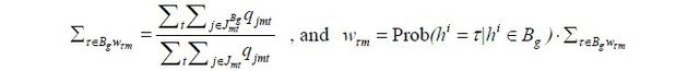
In order to take the effects of train availability on the distribution into account, and in attempt to reduce those effects, I assumed a uniform distribution within each time group (Bg). By extension, this assumption implies that hi is uniformly distributed within time group (Bg) but also that the train availability factor induces the observed hourly ridership.40 Therefore, Prob(hi∈Bg)= ∑τ∈Bg ϕτm in each city pair m is replaced with the proportion of rail passengers in city pair m traveling at time τ∈Bg, with the same number of travelers located at each point within Bg according to the assumption. Hence, ϕτm, the proportion of travelers who prefer to travel at during time period τ, is replaced with wτm such that
where  denotes the set of available trains in market mt whose schedule belongs to Bg and qjmt is the number of passengers purchasing j.41 Prob (hi=τ | hi∈Bg) is the distributions within the time group.42
Figure A1 shows the mean of the percentage of rail travelers who travel within an hour across city pairs (with bars) and the mean of proxies (with lines) for the distribution of travelers’ preferred travel times under the different assumptions of the time group distribution. Figures A1(a) and A1(b) show the distribution of hi based on six time groups and four time groups, respectively, combined with the uniform distribution regarding the within-time-group distributions. Figure A.1(c) displays the mean of two different proxies based on the four time groups, one using a Gaussian (with solid line) and one an arbitrary distribution (with dashed line) for the within-time-group distribution.
Column (3)-(6) of Table A1 and Panels B-E of Table A3 present the results from the specification that adopts wτm shown in (9) as a proxy for the distribution of hi. Column (3) and Panel B assume that B is partitioned into six time groups with four-hour intervals as defined in Appendix A.2, and that hi is uniformly distributed within each time group. Columns (4), (5) and (6) and Panels C, D and E assume that B is partitioned into four time groups with six-hour intervals as defined in Appendix A.2 with different within-group distributional assumptions for hi. Column (4) and Panel C utilize a uniform distribution, and Column (5) and Panel D use a normal distribution centered at the median of each time group. Column (6) and Panel E employ a randomly chosen arbitrary distribution, which is shown in Figure A1(c). Given that most of the losses resulting from schedule changes are due to the reduced number of scheduled trains and not due to reallocations, the implications regarding consumer welfare remain consistent with the findings from the main specification. They are robust across the assumptions regarding the distribution of hi. .
This paper is based on the third chapter of my Ph.D. dissertation. I am deeply indebted to professor Michael Riordan, Katherine Ho, and Chris Conlon for their advice and support. I would also like to thank Bernard Salanié, Brett Gordon, Emi Nakamura, and Yeon-Koo Che. The support for this research from Korail and the Korea Airport Corporation is gratefully acknowledged.
Trajtenberg (1989) proposes a method with which to measure product innovation, providing an example examination based on the social benefits from the innovation of CT scanners. Petrin (2002) quantifies the effects of the introduction of the minivan.
Spence (1976) demonstrates that firms tend to limit the number of products they offer by not introducing close substitutes for its existing products, leading to ambiguous implications regarding the introduction of new products on consumer welfare. Gabszewicz et al. (1986) illustrates how a monopolist would choose product quality if it can only produce a bounded number of products. The lesson to be learned from both of these analyses is that firms can react to the introduction of a new product by manipulating characteristics of the product other than the price.
This means Fare = Greater value among the Minimum Fare and (Rate per Km)·(Trip Distance). However, other types of price discrimination can be still offered to travelers. For example, the fares for weekdays are about 5% lower than those for weekends or holidays. There are also discount offers for group members, students, and senior citizens. Unfortunately, my data neither identifies weekend travelers from weekday travelers nor contains information on individual travelers; thus, any price discount or weekend surcharge would not be addressed throughout this paper.
For the detailed contents of the statutes applied to the Korail, please refer to the Railroad Enterprise Act and the Framework Act on the Development of Railroad Industry, which can be found on the website of the Ministry of Government Legislation (www.moleg.go.kr, in Korean) or on that of the Korea Legislation Research Institute (http://elaw.klri.re.kr/eng service/main.do, in English).
Travel by bus accounts for 70% of passenger transit, and air travel comprises only 4% of the market in Korea.
For example, a traveler may take train 1 from A0 to A5 and transfer to train 2 at A5 to arrive at B7. The product that the traveler purchases is then {(A0→A5,train 1), (A5→B7,train 2)}.
Douglas and Miller (1974) suggest two reasons why people cannot travel at their preferred times: the difference between a traveler's desired departure time and the closest scheduled departure; and delays due to excess demand during a traveler’s preferred travel time. This paper focuses more on the first source of compromise, which was referred to as frequency delay by Douglas and Miller (1974).
Unlike Douglas and Miller (1974), this paper does not consider capacity constraint as a source of schedule delay, but the train schedules.
I use departure time for ajmt, and adopt preference over departure time instead of arrival time in an alternative specification for the purpose of robustness check. The results are robust.
Berry et al. (2006) considers this as a factor of the preference of time to travel. I explicitly include the preference for the arrival or departure time in the model.
As discussed in Section III.A, the purpose of the trip can be to transfer to another mode of travel or to another train.
Although I assume hi to be an integer, it can be easily generalized to any of the 24 real numbers between 0 and 24.
According to Berry and Jia (2010), a mixture model with more than three types of consumers is difficult to estimate and sensitive to small changes in specifications or instruments.
This paper uses the “hour of the arrival time” for train schedules. The reason for
this is discussed in Section III.A, and thus  .
.
In other words,
where  . Figure 1 shows the mean percentage of rail travelers who travel within one hour across city
pairs (with bars) and the mean of the proxies (with lines) for the distribution of
travelers’ preferred travel times to illustrate the distribution of travelers’ preferred
times.
. Figure 1 shows the mean percentage of rail travelers who travel within one hour across city
pairs (with bars) and the mean of the proxies (with lines) for the distribution of
travelers’ preferred travel times to illustrate the distribution of travelers’ preferred
times.
The average number of Sae-ma-eul trains offered to the Group 2 city pairs in 2006 is understated because the number of city pairs where Sae-ma-eul trains stop in 2006 is greater than that from 2002. However, it is still significantly decreased because the average number of Sae-ma-eul trains offered in 2006 was 11; this number is not included in Table 2, even if the city pairs are limited to the 127 city pairs where Sae-ma-eul trains have been available since 2002.
Although the model in this paper does not include random coefficients, the existence of heterogeneous tastes for preferred times to travel makes the model similar to those with random coefficients.
For this paper, I transformed zmt using a principal component analysis of a given function h(∙) to make the columns of h(zmt) orthogonal.
For example, the rail company could schedule more trains at a popular time; thus, the schedule delay may be small for high-demand products.
For example, consider two cities, City 1 and City 2. Assume the cities have stations,
An1 and An2, respectively, both located on rail line A. Because people who travel from City 1 to City 2 would not care about routes An→ An’, ∀n,n’≠ n1 and ∀n,n’≠ n2, the demand for product j, given train t1, for An → An’ , ∀n,n’≠ n1 and ∀n,n’≠ n2 constitutes valid instrumental variables for j, with Rjmt representing such routes. For example, two of the instrumental variables are  where
where
 and
and
 .
.
While a city pair m is observed for multiple periods in the estimation, the products offered in a counterfactual
situation are observed for one period; thus,  is subscripted only with m. I take the mean of over months t within city pair m to compare it to .
The base category is the Mu-gung-hwa train. The mean utility of high-speed trains (KTX) is −0.41, which is lower than the mean utility of Sae-ma-eul of −0.05 for a 50 Km trip.
If there are two different routes which connect a city pair and one of the routes provides more frequent service, it is likely that the waiting time will be reduced, thereby inducing higher utility when choosing a route with more frequent trains as compared to other routes.
How a group is defined does not affect the demand estimates or the change in consumer surplus. The welfare analysis by group facilitates a clearer understanding of how heterogeneous consumers are differentially affected by the introduction of high-speed trains and the ensuing schedule changes.
The expected change from the schedule adjustment after high-speed trains were introduced is the sum of the changes caused by removing trains, adding trains and rescheduling trains.
Table 5 shows the summary statistics of (The per-person expected surplus changes in each market) × (Market Size).
Data used in the estimation covers 86 cities, and there are more than 150 bus terminals throughout the country, as obtained from the Korean Statistical Information Service, KOSIS.
The partition is defined based on the observation of the actual train schedule. The four groups are defined as 6:00-12:00, 12:00-18:00, 18:00-24:00, and 24:00-6:00, respectively.
This paper experiments different partitions with the length of the interval set to four hours instead of six hours; thus, the 24 numbers are partitioned into the six groups of 3:00-7:00, 7:00-11:00, 11:00-15:00 15:00-19:00 19:00-23:00, and 23:00-3:00.
. (1994). Estimating Discrete-choice Models of Product Differentiation. Rand Journal of Economics, 25(2), 242-262, https://doi.org/10.2307/2555829.
, , , & . (1986). Segmenting the Market: The Monopolist’s Optimal Product Mix. Journal of Economic Theory, 39, 273-289, https://doi.org/10.1016/0022-0531(86)90046-3.
. (2006). The Welfare Effects of Restricted Hospital Choice in the U.S. Medical Care Market. Journal of Applied Econometrics, 21, 1039-1079, https://doi.org/10.1002/jae.896.
, , & (2008). Schedule Delay Impacts on Air-travel Itinerary Demand. Transportation Research Part B, 42, 263-273, https://doi.org/10.1016/j.trb.2007.10.006.
(1972). A Time of Day Model for Aircraft Scheduling. Transportation Science, 6(3), 221-246, https://doi.org/10.1287/trsc.6.3.221.
. (2000). A Practitioner’s Guide to Estimation of Random Coefficients Logit Models of Demand. Journal of Economics & Management Strategy, 9(4), 513-548, https://doi.org/10.1162/105864000567954.
. (2003). New Products, Quality Changes, and Welfare Measures Computed from Estimated Demand Systems. Review of Economics and Statistics, 85(2), 266-275, https://doi.org/10.1162/003465303765299792.
. (1976). Product Selection, Fixed Costs, and Monopolistic Competition. The Review of Economic Studies, 43(2), 217-235, https://doi.org/10.2307/2297319.
. (1989). The Welfare Analysis of Product Innovations, with an Application to Computed Tomography Scanners. The Journal of Political Economy, 97(2), 444-479, https://doi.org/10.1086/261611.


 .
.
 .
.