I. Introduction

Household debt in Korea has steadily increased since the early 2000s, with the growth rate accelerating more rapidly since 2012. Accordingly, policymakers and researchers in Korea have been seriously concerned about the consistent increase in household debt. Those who claim that the current level of household debt is too high argue that large amounts of household debt can lead to a deterioration in economic growth (e.g., Cecchetti et al. 2011; IMF 2012; Bornhorst and Arranze (2013)). On the other hand, some argue that the general quality of household debt in Korea is moderate, as the majority of household debt is held by high-income and high-asset households (e.g., Hahm et al. 2010; Kim and Byun 2012; Kim and Yoo 2013).

In this paper, I analyze the household debt problem considering the aging population. More specifically, I examine how and why the household debt distribution by householder age group has changed over the past decade. It is well known that the elderly population has increased in Korea. Here, I analyze how the change in the demographic composition affects the household debt distribution by householder age. Moreover, I examine the effects of changes in household income and asset distribution on the change in the household debt distribution.

Initially, I compare Korea’s household debt distribution by the householder’s age to that of the US within and across time. The main motivation for comparing those two countries is that Korea’s household debt-to-GDP ratio in 2013 is nearly identical to that of the US for 2003 and 2013 (see Figure 1). The US ratio increased to almost 95% and later deleveraged after the global financial crisis. Korea’s household debt-to-GDP ratio, on the other hand, has not experienced any large adjustments, even after the global financial crisis. It is well known that US households took out much in loans, especially mortgages, before the financial crisis. Low-income and low-credit (or subprime-level) households could easily take out large amounts of loans before the economic crash (Mian and Sufi 2009; Keys et al. 2013; and others). By comparing the 2004 US household debt distribution, when loans were carelessly issued, to Korea’s recent household debt distribution, I can examine the risk level of the current Korean household debt problem, especially by age group.1 (Note that the aggregate levels of household debt-to-GDP ratios in both countries in these two years are nearly identical.) In addition, I examine household income, (net) assets, debt-to-income ratios, and debt-to-asset ratio distributions by householder’s age. By comprehensively analyzing household’s financial characteristics and comparing Korea to the US, I can evaluate the potential risks to Korean households.

FIGURE 1.

HOUSEHOLD DEBT-TO-GDP RATIOS FOR KOREA AND THE US

Note: Data are from the OECD and the Bank of Korea. Household debt data in the flow of funds table is used.

Next, I analyze how the household debt distribution by householder age group has changed over the last ten years (in the case of the US, I can examine changes over the last 20 years).2 The data shows that the proportion of household debt held by (relatively) younger households has decreased, while that of older households has increased over the last ten years. Specifically, the household debt distribution by the householder age group has shifted to the right. Moreover, the income, asset, and demographic distribution of households by householder age have all simultaneously shifted to the right. The shift in the income distribution is mainly driven by the changes in demographic factors. That is, as the proportion of older households increases, the proportion of income held by older households also increases. However, this explanation does not apply to household debt or asset distributions. Even after controlling for demographic factor, the proportion of household debt and assets held by young households has decreased, while that held by older households has increased. We can also observe such patterns in the US.

This motivates me to examine which factors mainly drive the change in the household debt distribution. More specifically, I consider household debt distribution by householder age group in 2004 and 20123 and analyze which household-specific characteristics affect changes in these distributions. Applying DiNardo et al. (1996), I consider a counter-factual 2004 household debt distribution where only the householder age distribution follows the distribution of 2012, while other household-specific characteristics remain in line with the 2004 distribution. By analyzing the results of this exercise, I can examine the effects of changes in householder’s demographic distribution over the last ten years on the household debt distribution. Similarly, I simulate a counter-factual scenario where only the household income (asset) distribution follows the distribution of 2012, with other household characteristics remaining in line with the 2004 distribution. Accordingly, the change in the householder demographic composition is the main driver behind the change in the household debt distribution by householder age. The demographic factor can explain the shift in the household debt distribution nearly by half. On the other hand, changes in either the income or asset distribution do not fully explain the change in the household debt distribution. I can also draw similar conclusions for the US, though the explanatory power of the change in the demographic composition is smaller than in Korea.

Given that demographic aging is an inevitable trend in Korea, as well as in the US, the proportion of household debt held by older households is also expected to increase. Hence, the Korean government must preemptively prepare for the household debt problem, especially for debt held by older households before the problem is exacerbated. Here, I propose policy directions which should be considered by the Korean government. First, the government should speed up the reforming of labor market inflexibility to prevent a sudden drop in household income when the householder reaches retirement age. Second, policymakers should monitor the possibility of asset price deflation more carefully. Third, household debt contracts in Korea should be restructured from the short-run bullet type to long-run amortization loans. Lastly, macro-prudential policies, such as debt-to-income (DTI) regulations, must be strengthened to spread the risk from unexpected adverse shocks.

There are many papers that analyze the potential risk of household debt in Korea. However, to the best of my knowledge, no studies have analyzed the structural risk of household debt which originates from an aging population. Kim and Byun (2012) analyzed individual-level debt distributions by income, credit score, occupation, financial intermediary type, age, and regional groups. Hahm et al. (2010) and Kim and Yoo (2013) also implemented a similar empirical exercise. Generally, these papers conclude that the current level of Korean household debt is not high enough to threaten the stability of financial system. However, certain types of households, such as low-income, non-banking debtors, are potentially vulnerable in negative stress scenarios. These papers commonly analyze household debt distributions by diverse debtor-specific characteristics at a certain time. Unlike those papers, I examine household debt distributions from a long-term perspective and analyze how and why the household debt distribution has changed structurally.

Other papers examine how household debt responds to unexpected exogenous shocks. Jeong and Kang (2013) analyzed household debt responses from unexpected changes in productivity (TFP), interest rates, or house prices. Justiniano et al. (2015) assert that the leverage and deleverage in US household debt is mainly driven by households’ taste for housing services. These papers commonly used a DSGE-style model and introduced certain exogenous shocks. My analysis regarding changes in household debt is driven more by a structural factor: changes in the demographic composition. In addition, this paper, unlike other papers, analyzes the household debt distribution rather than aggregate amounts (or levels) of household debt.

The remainder of this paper is organized as follows. Section II introduces the micro-data used in this paper. Section III compares Korea and US household debt distributions in a certain survey year (through a static comparison or a cross-section analysis). Section IV examines how the household debt distribution both in Korea and the US has changed over the last decade (via a dynamic comparison or a time-series analysis). Section V analyzes which factor(s) has (have) mainly driven the change in the household debt distribution over the past ten years. Finally, section VI concludes with policy implications.

II. Data Description

I used two household level micro-data to analyze the Korean household debt distribution: the Korean Labor and Income Panel Study (KLIPS) and the Survey of Household Finances and Living Conditions (SHFLC). KLIPS is a panel dataset which initiated in 1999. The most recently released survey was in 2012. SHFLC started in 2010, and the most recently updated survey was done in 2014. SHFLC is a panel structure between 2010 and 2011. Afterward, SHFLC re-sampled the interviewees in 2012, hence taking on a panel structure for the period of 2012 to 2014. SHFLC contains more finely categorized household asset and debt information than KLIPS. Unfortunately, because the initial survey year of SHFLC is 2010, I used KLIPS and SHFLC simultaneously to analyze the structural changes in the household debt distribution over the decade.

For the US case, I used the Survey of Consumer Finances (SCF) released by the Federal Reserve Board. SCF is similar to SHFLC, though with many more questionnaires. SCF has been released every three years, starting in 1983, and is not a panel dataset. Given that this paper analyzes the cross-sectional distributions of household debt over different years, a panel structure is not in fact necessary.4

Each dataset contains different household debt and asset categories. Hence, we need to clarify how aggregate household-level debt and assets are calculated. For KLIPS, household debt is the sum of financial debt (including secured and unsecured debt), non-financial debt, personal debt, jeonse5 deposits owed to renters, debt owed to mutual assistance society (or lodge money debt), and other loans. Similarly, aggregate household-level debt in SHFLC is defined by summing up the following components: financial debt, which includes both secured and unsecured debt; lodge money debt; debts related to credit cards; and jeonse deposits owed to renters. For SCF, total household debt is the sum of the following debt categories: mortgage/land contracts, debt related to investment real estate and vacation properties, business debt, vehicle loans, land contracts and notes (debt), credit card debt, home equity lines of credit, lines of credit not secured by residential property, education loans, other loans, loans for home improvement, other debt, margin loans, loans backed by insurance, and loans backed by pensions.

Similar to household debt, each dataset also defines household-level assets differently. For KLIPS, the sum of the housing value, jeonse deposits, and financial assets6 is defined as the household total assets.7 For SHFLC, household assets are calculated as the sum of financial assets, which includes all types of savings and financial investments, jeonse deposits, and real assets including real estate and non-real estate real assets. Household assets in SCF are defined by summing up the following components: the value of the primary residence, investment real estate and vacation properties; business equity; vehicles; financial assets;8 other assets; and land contracts and notes.

Table 1 summarizes household debt, income, assets, and net assets both in Korea and the US. The fraction of households that hold any type of debt (real-estate-related debt) in Korea is 65% (30%), while it is 77% (49%) and 75% (45%) in 2004 and 2013, respectively, in the US. Because it is meaningless to compare the levels of household debt between two countries, I measure the household debt burden by calculating the debt-to-income and the debt-to-asset ratios in both countries. The household debt-to-income ratio in Korea is 1.28 in 2014, while the ratio is 1.30 and 1.21 in 2004 and 2013, respectively, in the US.11 The household debt-to-income ratio conditional on having household debt is 1.68 in Korea, while it is 1.56 and 1.50 in 2004 and 2013, respectively, in the US. Hence, Korean households have slightly larger amounts of household debt in terms of their income than the US households. We can also observe even through the micro-level data that households in the US deleveraged their debts after the global financial crisis (in terms of their income).

TABLE 1

SUMMARY STATISTICS OF HOUSEHOLD DEBT, INCOME, AND ASSETS IN KOREA AND THE US

The household debt-to-asset ratio in Korea is 0.18, while the ratio in the US is 0.18 and 0.17 in 2004 and 2013, respectively. The household debt-to-asset ratio conditional on holding debt in Korea is 0.23, while it is 0.23 and 0.24 in 2004 and 2013, respectively, in the US. Household debt held by Korean households in terms of their assets is quite similar to that held by US households. Given that the average housing price in the US decreased significantly in the aftermath of the global financial crisis, the average household assets in the micro-level data also decreased by 6.3%. At the same time, US households also deleveraged their debt after the financial crisis, leading to identical US household debt-to-asset ratios in 2004 and 2013.

Using aggregate household debt statistics masks several important features and the potential vulnerability related to household debt in Korea. Hence, I examine the Korean household debt distribution and compare it to the distribution in the US. More specifically, I mainly focus on household debt distributions by householder age. It is well known that Korean society is aging, and the speed of this trend is more rapid than in any other OECD member country. The general trend is the same in the US, though the speed of population aging is slower. I sampled households in which the householder’s age is between 20 and 79, which covers nearly every household that carries on economic activities. It is known that the SCF data surveys very wealthy households. Hence, I dropped extremely rich or highly indebted US households when calculating statistical moments.12 (Specific explanations are in the footnotes of each figure and table in the next section.)

III. Static Analysis of Household Debt Distribution

In this section, I compare the 2014 Korean household debt distribution by householder age to the 2004 US household debt distribution. As shown in Figure 1, the recent household debt-to-GDP ratio in Korea is similar to the 2003 and 2013 ratios in the US. Before the global financial crisis, the US household debt increased monotonically. Next, US households deleveraged their debt through government-driven loan-modification programs, foreclosures, bankruptcies, and other measures (Gerardi and Li 2010 and Robinson 2009). Given that the 2014 Korea and 2004 US data are similar in terms of household debt-to-GDP ratio levels and their increasing trends, I initially choose those two years and compare the household debt distributions of two countries.

I define two measures which I mainly use in this paper to analyze household debt distributions by householder age. First, I calculate what portions of debt are held by a certain age group. Let m_i be the amount of debt held by household i , and w_i be the sample weight. Then, the proportion of debt held by a certain age group can be calculated as follows:

Under this measure, the debt-holding ratio by a certain age group may increase when the number of people in the age group is large enough. In order to control for an age-specific population effect, I define the second measure as shown below.

This is the ratio of the average debt held by a certain age group to the average debt held by the whole population. Hence, this ratio measures the relative amounts of debt held by a certain age group while controlling for demographic effects.

Figure 2 compares the 2014 Korea to the 2004 US household debt distributions by the householder age group. The left figure is the debt-holding ratio by householder’s age (Q_{Age group} ), and the right figure is the ratio of the average amount of debt held by a certain age to the average of all households ( P_{Age group} ). The older population in Korea holds a greater portion of the debt compared to this segment in the US, particularly those in their 50s. The debt of Korean households with householders in their 50s accounts for approximately 33% of all household debt, while it is 23% in the US, even lower than the debt held by those in their 40s. When I control for the demographic differences between Korea and the US, Korean household debt is comparatively more concentrated in the older-aged groups, particularly those in their 50s. Korean households with householders in their 50s are carrying 28% more debt than that held by the average household of the entire economy, which is higher by about 16% in the US. Due to the high proportion of the population in their 50s, along with the large amount of average debt, in Korea, the absolute proportion of their debts is much higher than that in the US.

FIGURE 2

Note: US Households with debt in the top 1% are dropped.

Source: (Korea) 2014 SHFLC; (US) 2004 SCF

Having large amounts of household debt may not be a serious problem if households have high enough income or asset simultaneously. In Figure 3, I present the household income distribution by householder age group. I similarly consider two measures: the proportion of household income held by a certain age group, and the ratio of the average income of a certain age group to the average of all households. The figure shows that Koreans experience a sharp decline in their incomes after their retirement age, implying that older people are more likely to face repayment and liquidity problems. The proportion of income earned by the population in their 50s in Korea is higher than that in the US, which is mainly attributed to population effects.

FIGURE 3

Note: US Households with incomes in the top 1% are dropped.

Source: (Korea) 2014 SHFLC; (US) 2004 SCF

Figure 4 reports the asset distribution by householder age. Older people in Korea own comparatively fewer assets than the same age group in the US. The average amounts of assets held by the older group, especially those in their 60s, are higher than those held by younger people both in Korea and the US. However, the average asset held by the older population in Korea is low relative to that in the US.

FIGURE 4

Note: US Households with assets in the top 1% are dropped.

Source: (Korea) 2014 SHFLC; (US) 2004 SCF

Similar to the asset distribution, older Koreans have lower amounts of net assets compared to the US households, as presented in Figure 5. Hence, these households in Korea, for whom income levels are also lower than those in the US, are more likely to be vulnerable to adverse asset price or liquidity shocks compared to their counterparts in the US.

FIGURE 5

Note: US Households with assets in the top 1% are dropped.

Source: (Korea) 2014 SHFLC; (US) 2004 SCF

FIGURE 6

Note: US households with either income or asset levels in the top 1% are dropped.

Source: (Korea) 2014 SHFLC; (US) 2004 SCF

In sum, Korea’s debt-to-income ratio increases as householders become older, unlike the US, and Korea’s debt-to-asset ratio does not decrease as rapidly as that of the US. The US debt-to-income ratio decreases as householders become older, as US people tend to borrow early in their lives and repay the debt throughout their life, including mortgages and education loans. On the other hand, the ratio in Korea is much higher than that in the US especially when people reach retirement age. Unlike the US, Korean households tend to take out loans without repaying the principal over their life cycle. Instead, they simply refinance the loans every 2-5 years, rolling over the debt again until their retirement age. In addition, a sudden drop in income after retirement age may be another factor which increases the debt burden of the older population in Korea. A similar interpretation can be applied to the debt-to-asset ratio. Because older Koreans have large amounts of debt even after their retirement age, along with lower assets than their US counterparts, the debt burden of older people, as evaluated by their assets, is greater in Korea.

IV. Dynamic Analysis of Household Debt Distribution

In the previous section, I examined household debt distributions during a certain survey year. In this section, I compare how the household debt distribution has changed over the last ten years (20 years in the case of the US). Then, I can analyze whether the household debt problem is a static (or time-invariant) or dynamic problem. If it turns out that the household debt distribution changes over time, we can estimate the potential change in the household debt distribution in the future and preemptively prepare policy measures to resolve the problem.

Figure 7 presents the Korean household debt distributions by householder age in 2004 and 2014. The proportion of debts held by older households has gradually increased over the last ten years, while the debt held by households less than 40 years of age had decreased. When I control for the effect of demographic changes, the average debt held by those in their 60-70s shows an increase, whereas that of the other age group shows a decrease. Hence, the Korean household debt distribution by householder age has shifted to the right over the last ten years.

FIGURE 7

Source: 2004 KLIPS and 2014 SHFLC

FIGURE 8

Note: US Households with debt in the top 1% are dropped.

Source: 1995, 2004, and 2013 SCF

The household debt distribution in the US also has shifted to the right over the last 20 years. The proportion of debt held by young households has decreased, while that held by older households has increased. When I control for demographic changes, the average household debt held by those in their 60-70s has increased, especially after the recent financial crisis.

I also examine the changes in household income distributions by householder age, as in the household debt distribution. The Korean household income distribution has similarly shifted to the right over the past ten years. That is, the proportion of household income held by those in their 50s has increased, while that held by those in their 30-40s has decreased over the past ten years. The change in the household income distribution is mainly driven by changes in the demographic compositions. As the number of older households increases, the portion of the total income held by these households also increases.

We can also observe similar patterns of changes in the household income distribution in the US. The proportion of the total household income held by young households has decreased, while that held by older households has increased. When I control for the demographic effects, the average household income (normalized by the average of all households) is nearly identical, especially between 1995 and 2004.

The proportion of household income held by older Korean households is much lower than that held by their counterpart group in the US. In addition, the average amount of income for Korea’s older households is much lower than that in the US. This pattern is also found nearly ten years ago. Hence, the fact that Korean households, on average, tend to experience a steep decline in their income once they retire from their jobs is a persistent problem which has not recently been demonstrated.

FIGURE 9

Source: 2004 KLIPS and 2014 SHFLC

FIGURE 10

Note: US Households with incomes in the top 1% are dropped.

Source: 1995, 2004, and 2013 SCF

Household assets held by older Korean households have increased slightly over time. However, the proportion of assets held by older Korean households is much lower than that in the US. At the same time, the average asset level is lower in Korea compared to the US.

In sum, the proportion of household debt held by each age group has shifted over the last ten years. At the same time, the distributions of household income and assets have also shifted to the right. Therefore, when we prepare policy measures to resolve the household debt problem, we must understand the nature of the household debt distribution, which is not time-invariant. In the following section, I analyze why the household debt distribution has shifted both in Korea and in the US. In turn, I examine estimated changes in the household debt distribution in the near future and draw policy implications.

FIGURE 11

Source: 2004 KLIPS and 2014 SHFLC

FIGURE 12

Note: US Households with assets in the top 1% are dropped.

Source: 1995, 2004, and 2013 SCF

V. Analyzing the Driving Forces behind the Changes in the Household Debt Distribution

In the previous section, I found that household debt, income, and asset distributions by householder age group have shifted over the past ten years. In this section, I analyze the main driving force that has shifted the household debt distribution. More specifically, I analyze whether changes in demographic (or age), income, or asset distributions have shifted household debt distributions, as well as how much each component has contributed to the shift. This analysis is based on DiNardo, Fortin, and Lemieux (1996) and its application.

A. Analysis Methodology

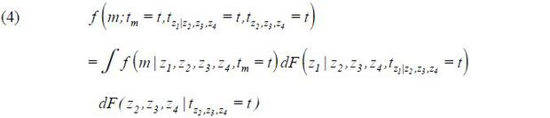
Let (m_i , z_i , t) be an observation specific to household i , where m is the amount of household debt, z denotes the household-specific characteristics, and t is a (survey) year which takes only two values to examine the change in the distribution from the initial to the terminal year of the analysis. Let f_t(m) be household debt density function (pdf) at time t . The unconditional household debt density function can then be rewritten as follows:

That is, the unconditional density, f_t(m) , is the integral of the conditional density of household debt at time t_m over the distribution of the household characteristics density function dF (z | t_z = t) at time t_z .

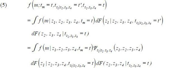
Suppose that the household characteristics z is composed of four components: the householder age (z₁) , income (z₂) , asset (z₃) , and other characteristics (z₄) . That is, z = (z₁ ,z₂ ,z₃ ,z₄ ) . Then, we can rewrite the above density function as follows:

Following the notation of DiNardo et al. (1996), we consider a counter-factual time t household debt density for which the household characteristics except for z₁ remain at their t -year and the z₁ distribution is switched to their t' -year where t ≠ t' . For example, we can imagine a hypothetical 2004 ( t ) household debt distribution in which only the householder’s age distribution follows their 2012 ( t' ) and all other household characteristics distributions remain at their 2004 ( t ). Such a counter-factual density can be written as

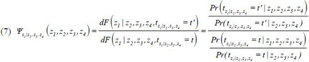
where Ψ_z1|z2.z3.z4 (z₁,z₂,z₃,z₄) is a weighting function defined by

The only difference between the original household debt density function and the counter-factual density function is the weight function, Ψ_z1|z2.z3.z4 (z₁,z₂,z₃,z₄). The weighting function can be reorganized using Bayes’ rule, as follows:

In the actual computation, I used the probit model to solve the last term of the above equation. That is, dummy variables are generated, which are 1 if the data year is t' and 0 otherwise. Similarly, another dummy variable is generated, which is 1 if the data year is t and 0 otherwise. In such a case, for example, the weighting function can be calculated as follows:

In the actual implementation, I used the age of the household head, the square of his/her age, log real assets, log real income, an education dummy (1 if less than a high school degree, 0 otherwise), homeownership status, and the number of household members.

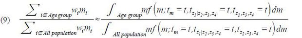
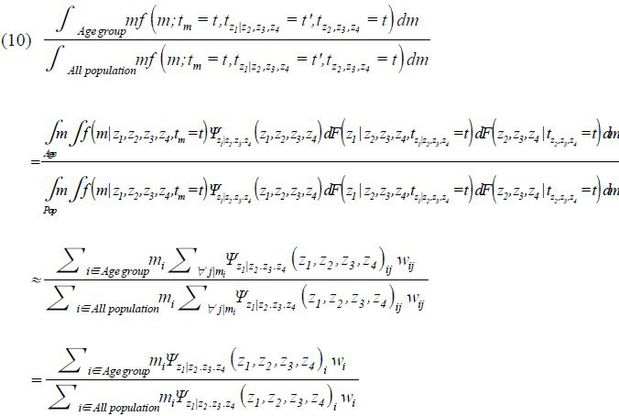
Because I mainly analyzed how the household debt distribution by householder age changes over time, it is necessary to manipulate the unconditional density function to obtain the household debt distribution by householder age group. The portion of household debt held by each age group can be rewritten as follows:

Similarly, we consider the counter-factual time- t household debt distribution by householder age where only the z₁ distribution changes of their time- t' and other household characteristics remain at their time- t .

Therefore, the counter-factual household debt distribution by householder age can be calculated using the newly defined weighting function, Ψ_{z1|z2.z3 .z4} (z₁,z₂,z₃,z₄).

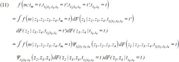
Here, I only consider cases in which only the distribution of z₁ changes to the year t' . We can also extend the household debt density function where the distribution of z₁ and z₂ both change to the year t' , while the other characteristics remain at time t . Then, the counter-factual unconditional density function can be written as follows,

where the additional weighting function can be defined by

The other procedures are identical to those used earlier. The only difference is that the new weighting function when calculating the household debt distribution by householder age is Ψ_z1|z2.z3.z4 (z₁,z₂,z₃,z₄)Ψ_z2|z3.z4(z₂,z₃,z₄)w, rather than Ψ_z1|z2.z3.z4 (z₁,z₂,z₃,z₄)w.

Before presenting numerical results, several factors should be noted with regard to the methodology presented here.13 The spirit of the methodology is similar to that of Oaxaca (1973). However, the Oaxaca decomposition mainly focuses on how the average of a variable (e.g., the average household debt) would change if the average of a certain explanatory variable (e.g., the average householder’s age) changes, ceteris paribus. Unlike Oaxaca’s methodology, DiNardo et al. (1996) focused on changes in the overall density if the distribution of explanatory variable(s) changes, ceteris paribus. As noted in DiNardo et al. (1996), this method cannot take into account the general equilibrium effect of a change in the explanatory variable(s). For example, when the household demographic distribution changes, the household asset or income distribution would change, in turn indirectly affecting the household debt distribution. This methodology cannot take into account such an indirect effect from changes in the density of explanatory variables.

B. Results

In this subsection, I analyze how changes in the distribution of household-specific characteristics affect the household debt distribution by householder age group. As presented in the previous section, the household debt distribution has shifted to the right over the past ten years. At the same time, household demographics, income, and asset distributions have also changed. Among those changes, I examine which factors mainly affect changes in the household debt distribution, based on the methodology suggested in the previous subsection.

I choose two survey years, 2004 and 2012, using the KLIPS data.14 First, I consider a counter-factual scenario in which only household demographic (or age) distributions change to those of 2012, while other household characteristics remain at 2004. By analyzing such a counter-factual scenario, I could analyze how changes in demographic distributions contribute to changes in household debt distributions. The top left figure in Figure 13 shows that changes in the demographic distribution from 2004 to 2012 contribute to the change in the household debt distribution by nearly half (see the dotted line). A change in the household income distribution also slightly affects the change in the household debt distribution (see the top right figure). However, the effect of the change in the income distribution is smaller than that caused by the change in the demographic distribution. A change in the asset distribution has almost no effect on the household debt distribution (see the bottom left figure). Simultaneous changes in household income and demographic distributions from 2004 to 2012 cause the 2004 household debt distribution nearly to converge to the 2012 distribution. Therefore, a change in the demographic distribution, partly in conjunction with a change in the income distribution, is the main driving force which has shifted the Korean household debt distribution over the last ten years.

To measure quantitatively how changes in each household characteristic explain changes in the household debt distribution, it is necessary to define the “distance” measure between two different densities. Let g be the (conditional) density function of household debt by householder age.15 Let g_t be the household debt distribution at time t , and g_z be the counter-factual household debt distribution where only the household characteristic z follows the 2012 distribution while other household characteristics remain at their 2004. The Figure 13 shows a visual representation of the density functions of g₀₄(age) , g₁₂(age) , and g_z(age) , where z ∈{age, income, asset, income and age}. I define the measure of the distance between two densities as follows:16

FIGURE 13.

CHANGES IN THE HOUSEHOLD DEBT DISTRIBUTION BETWEEN 2004 AND 2012 DRIVEN BY EITHER AGE, INCOME, OR ASSET DISTRIBUTION CHANGES

Source: 2004 and 2012 KLIPS

The explanatory power of the change in the household debt distribution attributed to household characteristics z is then measured as follows:

If the change in the household characteristic z fully shifts the 2004 household debt distribution to 2012, the measure D_{z, 12} would be 0. Hence, the explanatory power of z is 100%. On the other hand, if the household characteristic z cannot explain any shift in the household debt distribution between 2004 and 2012, the measure D_{z, 12} would be equal to D_{04, 12} . Hence, the explanatory power of z is zero.

Table 2 reports how each combination of household characteristics can explain changes in the household debt distribution between 2004 and 2012. A change in the demographic distribution can explain a change in the household debt distribution by nearly half. A change in the income (asset) distribution can explain a change in the household debt distribution by 24.8% (3.5%). Simultaneous changes in the household age, income, and asset distributions can explain changes in the household debt distribution by 64%. However, there remains 36% of the change in the household debt distribution which is not explained by simultaneous changes in the household age, income, and asset distributions. I suspect that changes in the financial market environment or household-specific idiosyncratic shocks may account for this unexplained gap.

TABLE 2

DECOMPOSING CHANGES IN THE KOREAN HOUSEHOLD DEBT DISTRIBUTION BY HOUSEHOLD CHARACTERISTICS

This leads to the question of how much household income, asset, and demographic distributions have changed over the last 10 years. Figure 14 presents the kernel density of the log real household income, log real assets, and the age distribution. Household income and asset distributions have slightly shifted to the right, which partly reflect the (real) growth in the Korean economy. Not surprisingly, the householder age distribution has shifted to the right visibly. Though household asset, income, and age distributions have all shifted over the last ten years, the change in the household debt distribution is mainly explained by the change in the age distribution.

FIGURE 14

Note: A Gaussian kernel function is used.

Source: 2004 and 2012 KLIPS

I can draw similar results for the US. As shown in Figure 15, the change in the demographic distribution partly affects the change in the household debt distribution by householder age. However, changes in the household income and asset distributions have nearly no effect on changes in the household debt distribution.

FIGURE 15.

CHANGES IN THE HOUSEHOLD DEBT DISTRIBUTION BETWEEN 2004 AND 2013 DRIVEN BY EITHER AGE, INCOME, OR ASSET DISTRIBUTION CHANGES

Source: 2004 and 2013 SCF

Table 3 reports that a change in the demographic distribution can explain a change in the household debt distribution by 44%. However, changes in either the income or asset distribution have negligible explanatory power. Hence, the change in the household debt distribution over the last decade in the US is mainly driven by the change in the demographic distribution, as it was in Korea.

TABLE 3

DECOMPOSING CHANGES IN THE US HOUSEHOLD DEBT DISTRIBUTION BY HOUSEHOLD CHARACTERISTICS

Between 2004 and 2013, the US economy experienced an unprecedented boom and bust, especially in the housing market. More specifically, US financial intermediaries lent money to households with (relatively) lax screening efforts, which contributed to the boost in the housing market (Keys et al. (2013)). As a result, many subprime loans were issued, which triggered and exacerbated the financial crisis starting in 2007. After the crisis, the US government implemented many government-driven mortgage modification programs, which partly reduced the household financial burden. Given that the US economy experienced numerous events over the last ten years, explaining the change in the household debt distribution simply with household-specific characteristics may not be successful.

Kernel densities of the log real income, real asset, and age distributions are presented in Figure 16. The income and asset distributions have not changed significantly over the last ten years. However, we can observe that the US population is also aging. Hence, the change in the household demographic distribution is also an important factor which explains the shift in the household debt distribution in the US, as it does in Korea.

FIGURE 16

Note: A Gaussian kernel function is used.

Source: 2004 and 2013 SCF

VI. Concluding Remarks

In this paper, I analyze how household debt distribution in Korea and the US has changed over the last ten years. Household debt distribution by householder’s age in both countries has shifted to the right. My analysis shows that the shift in the household debt distribution is mainly driven by a change in householder’s demographic distribution, especially for Korea. Changes in either household income or asset distribution cannot successfully explain the shift in the household debt distribution. For the US, the change in demographic distribution can partly, though not enough, explain the change in the household debt distribution.

One possible reason why the demographic factor has a strong power in explaining the shift in the household debt distribution in Korea is the Korean-specific debt contract structure. Most mortgage and non-mortgage debt contracts in Korea are short-term and bullet-type loans. That is, households tend to take out loans with a 2-5 year contract period. And then, they repay nothing or pay only interests while in their contract duration. When it comes to the contract expiration date, households refinance loans again, with contract periods of 2-5 years. Hence, the loan principal does not decrease as time goes on and is rolled over repeatedly, with simply paying back the interest. This allows us to observe the cohort effect in debt distribution over the long-time.

On the contrary, the debt contract structure in the US is quite different. Households tend to take out loans, especially mortgages, with a long-term horizon. They then pay back both interest and principal over their life cycle. In turn, household net equity increases as householders become older. This explains why the demographic effect which explains the change in the household debt distribution is not as strong as in the Korean case. In addition, the US economy has experienced a housing/asset boom and bust over the last ten years. Hence, it is difficult to explain the full shift in the household debt distribution merely according to the change in the distribution of demographic or household-specific characteristics.17

We can draw the following policy implications for the Korean economy from this analysis. First, as Korean people become older, the proportion of household debt held by older households is expected to increase more in the near future.18 If older households have large amounts of assets and incomes, the household debt problem will not be serious. However, as presented in the main text, householder income levels for those in their 60-70s suddenly decrease. In turn, it is highly probable that older householders may experience more severe liquidity problems as they become older, along with their debt principal burden. Furthermore, the large portion of the income earned by older Koreans comes from either wages or income from businesses, while these households in the US mostly earn their income from social security, pensions, and annuities (or public transfers).19 That is, the incomes earned by Korean seniors are less secure and stable than those earned by their US counterparts. Therefore, policymakers need to consider diverse measures to improve and stabilize old-aged income. One possible way may be a structural change in the labor market which extends the retirement age of workers through the implementation of a wage peak system. In a similar vein, due to the seniority-based wage system in the current Korean labor market, older employees are unable to avoid early retirement and become self-employed, which in general leads to a sudden decrease in their incomes.

Second, Korean policymakers need to monitor the possibility of asset price deflation more carefully. Many researchers have found that Korean household debt problems will not shift toward systematic risk because Korean households have enough assets, providing a safe buffer for the debt problem. If Korean asset prices are deflated for some exogenous reasons, financial intermediaries may force households to pay back their debt, as their collateral value also decreases. In such a case, it is possible that households will start selling their assets in the market to pay back their remaining debt burden, which in turn would lead to a decrease in asset prices again. The worst scenario may be a collapse in asset values along with a sudden increase in household defaults. In order to avoid such a sudden drop in asset values while preserving a certain level of income for senior citizens, policymakers can consider an extension of asset-backed security markets or reverse mortgage programs. These programs may reduce the likelihood of a sudden drop in asset prices while preventing an abrupt decrease in the incomes of older households.

Third, policy efforts should be strengthened to make a transition in the debt contract structure from short-term bullet-type to long-term amortized loans. As mentioned earlier, Korean households tend to roll over their debt without reducing their principal. This phenomenon is possible due to the prevalence of short-term bullet-type loans. Under an economy in which asset (or housing) values consistently increase, this type of loan contract structure is sustainable. That is, households have capital gain opportunities with a constant (nominal) value of debt. Hence, even when householders retire, experiencing a steep decrease in their incomes, they have already accumulated high enough levels of net assets while young. However, as the Korean economy has become more developed, the chances for capital gain have narrowed. Under this environment, households that take out loans without reducing their debt levels have little chance to realize capital gains (or increased net asset holdings) when they retire. Because retired households tend to experience a serious decrease in their incomes, these households may face both liquidity and net asset shocks. This motivates why Korean policymakers should seriously consider a change in the debt contract structure. By inducing Korean households to pay back their debts over their life cycle, as is done the US households, older Korean households can retire from their jobs without concern over their remaining debt, even when their incomes after retirement suddenly decrease.

In sum, the household debt problem in Korea is partly a structural problem originating from the change in the demographic composition. It is difficult to avoid or reverse the changes in demographic trends. However, the Korean government can avoid potential system risk by strengthening macro-prudential policies and through labor market restructuring, asset market monitoring, enacting changes in debt contract structures, and other means. It is well known that Korea’s speed of population aging is the fastest among OECD member countries. I recommend that the Korean government take action as soon as possible before the problem worsens.