
Time-varying Cointegration Models and Exchange Rate Predictability in Korea
Abstract
We examine the validity of popular exchange rate models such as the purchasing power parity (PPP) hypothesis and the monetary model for Korean won/US dollar exchange rate. Various specification tests demonstrate that Korean data are more favorable for both models based on time-varying cointegration coefficients as compared to those based on constant cointegration coefficients. When the abilities to predict future exchange rates between those models based on time-varying cointegration coefficients are compared, an in-sample analysis shows that the time-varying PPP (monetary model) has better predictive power over horizons shorter (longer) than one year. Results from an out-of-sample analysis indicate that the time-varying PPP outperforms models based on constant cointegration coefficients when predicting future exchange rate changes in the long run.
Keywords
Exchange rate, Monetary model, Predictability, Purchasing power parity, Time-varying cointegration
JEL Code
F37, F41
I. Introduction
Understanding the movements of exchange rates is important, especially in Korea, where exports play an influential role in her growth. In spite of the importance of exchange rates, however, understanding the movements of exchange rates based on macroeconomic models has been a challenge to economists. Hence, the goal of this paper is to examine whether popular macroeconomic models such as the Purchasing Power Parity hypothesis (henceforth PPP) and/or the monetary model can explain fluctuations in the Korean won/US dollar exchange rate. More specifically, we investigate which model between the PPP hypothesis and the monetary model provides a better tool for understanding exchange rate fluctuations in Korea. In order to achieve this goal, we relate the exchange rate to macroeconomic variables based on the concept of cointegration. The cointegration approach has been widely applied in the literature on exchange rates since its introduction by Engle and Granger (1987). However, the cointegration relationships presented in this study include the constant cointegration relationship, which has been examined in many studies, as well as the type of cointegration relationship which allows cointegration coefficients to vary gradually over time.
There are reasons why we analyze the time-varying cointegration relationship between the exchange rate and macroeconomic variables in addition to the constant cointegration relationship between those variables. Many empirical studies have reported that the structure of the money market has changed over time.1 Cheung and Chinn (2001) also show that the macroeconomic variables and economic models utilized by foreign exchange traders to understand exchange rate movements shift over time. Bacchetta and van Wincoop (2013) demonstrate that the relationship between the exchange rate and macroeconomic variables varies over time when the pertinent structural parameters are unknown. Finally, Bierens and Martins (2010) and Park and Park (2013) provide evidence of time-varying cointegration relationships among variables under the PPP hypothesis and among variables under the monetary model, respectively.
Most of the above-mentioned studies, however, focus on the US or other advanced economies.2 In addition to the reasons discussed above, considering the time-varying cointegration relationship is particularly relevant in Korea because her economic structure has changed over time. These structural changes include financial and economic reforms suggested by International Monetary Fund (IMF) during the Asian Financial Crisis of 1997 as well as various currency swap agreements during the Global Financial Crisis. Given that these reforms and agreements must result in gradual changes in the economic environment in which the exchange rate and other macroeconomic variables are determined, it is a meaningful exercise to extend the time-varying cointegration approach to the won-dollar exchange rate in Korea under both the PPP hypothesis and the monetary model.
The paper is organized as follows. Section II briefly presents both the PPP hypothesis and the monetary model. Section III provides a discussion of the data and the econometric methodology of the time-varying cointegration approach. Section IV reports that the PPP hypothesis and the monetary model based on the constant cointegration approach are limited in terms of being able to explain the movements of the exchange rate in Korea. Section V shows that Korean data are more favorable when used with the PPP and the monetary model based on the time-varying cointegration approach through various model specification tests. Section VI compares the capability to predict future exchange rate changes among the time-varying PPP, the time-varying monetary model, and a combination of the The paper is organized as follows. Section II briefly presents both the PPP hypothesis and the monetary model. Section III provides a discussion of the data and the econometric methodology of the time-varying cointegration approach. Section IV reports that the PPP hypothesis and the monetary model based on the constant cointegration approach are limited in terms of being able to explain the movements of the exchange rate in Korea. Section V shows that Korean data are more favorable when used with the PPP and the monetary model based on the time-varying cointegration approach through various model specification tests. Section VI compares the capability to predict future exchange rate changes among the time-varying PPP, the time-varying monetary model, and a combination of the two via in-sample and out-of-sample analyses. The in-sample analysis shows that the time-varying PPP shows better predictive power over horizons shorter than one year, whereas the time-varying monetary model outperforms when the horizons are longer than one year. The time-varying PPP shows better performance according to the results of the out-of-sample analysis. Concluding remarks are offered in Section VII.
II. Theoretical Discussion: PPP and Monetary Model
In this section, we present a brief discussion of the PPP hypothesis and the monetary model, and derive the time-varying cointegration version of these models.
A. Purchasing Power Parity (PPP)
The PPP hypothesis states that when goods are traded freely, the nominal exchange rate adjusts so that the goods must sell for the same price in both countries. This idea can be expressed by the following equation,

where St is the nominal exchange rate, Pt is the domestic price level (i.e., in Korea), and  is the foreign price level (i.e., in the US). A is a constant which captures trade barriers and difference in preferences between
the two countries. When temporary deviations from the PPP relationship is allowed,
Equation (1) can be re-expressed after taking logarithms, as follows:
is the foreign price level (i.e., in the US). A is a constant which captures trade barriers and difference in preferences between
the two countries. When temporary deviations from the PPP relationship is allowed,
Equation (1) can be re-expressed after taking logarithms, as follows:

where lower letters denote the logarithms of the corresponding capital letters, and
εt represents temporary deviations from the PPP. Although st and  are known to be I(1) variables,
  must be stationary under the PPP, which implies a [1, −1] cointegration vector for
the exchange rate and relative price. Many empirical studies have examined the validity
of the PPP under constant cointegration coefficients, providing evidence that the
PPP does not hold in most cases. However, this failure of the PPP may be due to the
fact that the constant cointegration coefficient cannot reflect gradual changes in
economies as opposed to a failure of the PPP in general. Hence, we also consider the
following PPP relationship based on the time-varying cointegration coefficient,
must be stationary under the PPP, which implies a [1, −1] cointegration vector for
the exchange rate and relative price. Many empirical studies have examined the validity
of the PPP under constant cointegration coefficients, providing evidence that the
PPP does not hold in most cases. However, this failure of the PPP may be due to the
fact that the constant cointegration coefficient cannot reflect gradual changes in
economies as opposed to a failure of the PPP in general. Hence, we also consider the
following PPP relationship based on the time-varying cointegration coefficient,

where βt is the cointegration coefficient which varies smoothly over time, capturing the effect of gradual changes in the economic environment on the PPP relationship.
B. Monetary Model
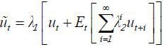
The monetary model has been examined in many studies, and there has been some debate regarding whether it accurately explains fluctuations in exchange rates. For example, Mark (1995) and Chinn and Meese (1995) show that the monetary model has significant predictive power for exchange rate movements, whereas Kilian (1999) and Berkowitz and Giorgianni (2001) provide evidence against exchange rate predictability based on the monetary model. The traditional monetary model examined in these studies can be summarized by the following four equations:


where mt and yt are the logarithms of the money supply and real income level, respectively. it is the level of the nominal interest rate. πt is the deviation from uncovered interest parity (UIP) or the unobserved risk premium,
while vt and  denote unobserved velocity shocks. We assume that πt , vt and follow stationary processes.3 γ and ϕ correspondingly represent the elasticity of the money-demand income and the semi-elasticity
of the money-demand interest rate. Under the assumption of
denote unobserved velocity shocks. We assume that πt , vt and follow stationary processes.3 γ and ϕ correspondingly represent the elasticity of the money-demand income and the semi-elasticity
of the money-demand interest rate. Under the assumption of  and
and  , these four equations can be combined to express the following cointegration relationship
between st,
, these four equations can be combined to express the following cointegration relationship
between st,  and
and  :
:

Where  ,
,  ,
,  , and
, and 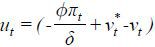 . Equation (8) implies the
 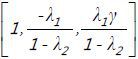 cointegration vector for st, , and , and this constant cointegration vector becomes [1, -1, 1] under the assumption of
β = δ = γ =1 .
cointegration vector for st, , and , and this constant cointegration vector becomes [1, -1, 1] under the assumption of
β = δ = γ =1 .
As shown in Park and Park (2013), however, data in advanced economies are not favorable when used with the monetary model based on constant cointegration coefficients. Hence, when the underlying parameters (δ, β, ϕ, and γ) are allowed to vary over time, we can derive the following time-varying cointegration relationship:

where 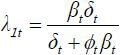 ,
, 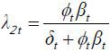 ,
,  and
and 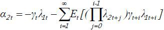 .
.
III. Data and Econometric Methodology
A. Data
This study ascertains the validity of the PPP and monetary model in Korea. As a result, empirical analyses require data for the exchange rate (Korean won per US dollar) and data for macroeconomic variables such as the price index, money supply and real income levels for Korea and the US. Because the frequency of the data utilized in the analyses is monthly, industrial production is used for real income in both countries.4 The M1 money stock and the Consumer Price Index (CPI) are used for the money supply and price-level variables.5 Data for Korea and the US are obtained from the websites of the Bank of Korea and the Federal Reserve Bank of St. Louis, respectively.6 The data of the money supply and real income levels are seasonally adjusted, and the sample period covers the period between January of 1980 and April of 2015.
B. Econometric Methodology
Considering that the cointegration approach under constant cointegration is widely applied in empirical studies, we introduce briefly the time-varying cointegration approach as proposed by Park and Hahn (1999) in this subsection. Suppose that the following time-varying cointegration relationship holds between st , x1t , and x2t ,

where ut denotes the cointegration residuals and ρ1t and ρ2t are the time-varying cointegration coefficients.
Define smooth functions ρ1 and ρ2 on [0, 1] such that  and
and  , where T is the sample size. Under the assumption that ρ1 and ρ2 are smooth enough so that they can be approximated by a series of polynomials and/or
trigonometric functions, Equation (10) can be written as follows:
, where T is the sample size. Under the assumption that ρ1 and ρ2 are smooth enough so that they can be approximated by a series of polynomials and/or
trigonometric functions, Equation (10) can be written as follows:
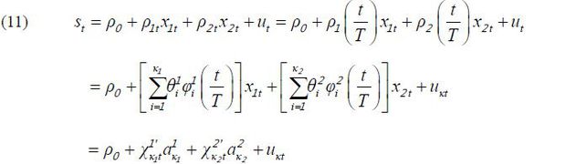
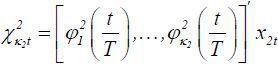
Where  and
and  are the corresponding series functions used to approximate ρ1 and ρ2 ,
 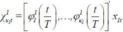 ,
,  ,
, 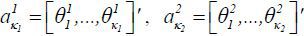 , and
, and 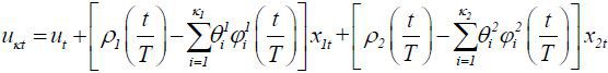 .
.
When st , x1t , and x2t are nonstationary, canonical cointegration regression (CCR) offers better asymptotic results. Hence, Equation (11) under the CCR transformation becomes

Where  ,
,  , and the superscript † denotes CCR transformed variables. Once the LS estimators for
  and
and  in Equation (12) are obtained, ρ1 and ρ2 can then be approximated by
  and
and  , respectively. Fourier Flexible Form (FFF) series functions, which include polynomials
and trigonometric functions, are utilized to approximate ρ1 and ρ2 .
, respectively. Fourier Flexible Form (FFF) series functions, which include polynomials
and trigonometric functions, are utilized to approximate ρ1 and ρ2 .
IV. Assessment of Macroeconomic Models with Constant Cointegration Coefficients
Before beginning any analysis to examine a cointegration relationship, we check whether variables under the PPP or monetary model are indeed nonstationary in Korea, as they are in other countries. For this purpose, we use the Augmented Dickey-Fuller (ADF) test and the Kwiatkowski-Phillips-Schmidt-Shin (KPSS) test for both the level and the first difference of the exchange rate, relative money, relative income and relative price. As shown in Table 1, the unit root null hypothesis of the ADF test cannot be rejected for those variables in levels, while the unit root null hypothesis is rejected in the first difference of the variables. Furthermore, the stationarity null hypothesis of the KPSS test can be rejected for all of these variables in levels, whereas the stationarity null hypothesis is not rejected for any of the variables in the first difference. These results, shown in Table 1, strongly suggest that all of the variables under the PPP or the monetary model can be considered to be integrated of order one individually.
TABLE 1
UNIT ROOT TESTS FOR VARIABLES IN THE MONETARY MODEL AND PPP
Note: Numbers in parentheses are the MacKinnon (1996) one-sided p-values for the ADF test statistics. Each lag length is determined by the Akaike information criterion (AIC). The null hypothesis of the Kwiatkowski-Phillips-Schmidt-Shin test is of stationarity and the alternative is the presence of a unit root. The asymptotic critical value for the test statistics is from Kwiatkowski-Phillips-Schmidt-Shin (2002), and it is 0.146 at the 5% level.
A. The PPP hypothesis with constant cointegration coefficients
In order to assess the capability of the PPP hypothesis to explain movements of the
exchange rate in Korea, we initially examine whether  is stationary. That is, we investigate the validity of the [1, −1] cointegration
vector between st and
is stationary. That is, we investigate the validity of the [1, −1] cointegration
vector between st and  . Hence, the ADF test is conducted for
  . As shown in Table 2, the unit root null hypothesis can be rejected marginally for . This implies that there exists a long-run relationship between st and based on the [1, −1] cointegration vector.
TABLE 2
ASSESSMENT OF THE PPP WITH CONSTANT COINTEGRATION COEFFICIENTS
Note: For the Engle-Granger test,  is run in the first step, after which the ADF test is conducted for the residuals
in the first step. The critical value for the ADF statistic is from Phillips and Ouliaris (1990). For the Johansen test, when the ‘no cointegration’ null is tested, a linear deterministic
trend in the data is allowed and the computation of the critical values is based on
MacKinnon-Haug-Michelis (1999) p-values. Lag intervals are selected by the AIC.
is run in the first step, after which the ADF test is conducted for the residuals
in the first step. The critical value for the ADF statistic is from Phillips and Ouliaris (1990). For the Johansen test, when the ‘no cointegration’ null is tested, a linear deterministic
trend in the data is allowed and the computation of the critical values is based on
MacKinnon-Haug-Michelis (1999) p-values. Lag intervals are selected by the AIC.
When we remove the restriction on the cointegration vector, however, the plausibility
of the PPP hypothesis is altered. That is, we subsequently address whether there exists
any other constant cointegration vector between st and rather than [1, −1]. For this purpose, the Engle-Granger test is conducted. The estimated
cointegration coefficients between st and in the first step of the Engle-Granger test are as follows:

-
-
where numbers in parentheses are standard errors.7
-
The estimated cointegration vector is [1, −1.19]. Although the estimated coefficient is highly significant, the ADF test for the residuals from the first step of the Engle-Granger test states that the unit root null hypothesis cannot be rejected at the 5% level, as shown in Table 2. In addition to the Engle-Granger test, the cointegration test proposed by Johansen (1988) and Johansen and Juselius (1990) is considered in the last four rows of Table 2. Regardless of whether the trace statistic or the maximum eigenvalue statistic is used, the null of no cointegration cannot be rejected. Moreover, the results do not depend on whether the trend is added in the test or not.
The results in Table 2 are somewhat odd due to the following reason. The PPP with the restriction on the cointegration vector ([1, −1]) has some support from the data, but the constant cointegration PPP without the restriction does not. These somewhat odd results in Table 2 suggest that the PPP hypothesis based on the constant cointegration relationship has limited ability to explain the exchange rate in Korea.
B. The monetary model with constant cointegration coefficie
Similarly to the examination of the PPP hypothesis in the previous subsection, we
first check whether  is stationary under the assumption of β = δ = γ = 1 . Hence, the ADF test is conducted for
  . As shown in Table 3, the unit root null hypothesis cannot be rejected for This implies that we cannot find a long-run relationship between st, and based on the [1, −1, 1] cointegration vector.
TABLE 3
ASSESSMENT OF THE MONETARY MODEL WITH CONSTANT COINTEGRATION COEFFICIENTS
Note: For the Engle-Granger test,  is run in the first step and the ADF test is then conducted for the residuals in
the first step. The critical value for the ADF statistic is from Phillips and Ouliaris (1990). For the Johansen test, when the ‘no cointegration’ null is tested, a linear deterministic
trend in the data is allowed and the computation of the critical values is based on
MacKinnon-Haug-Michelis (1999) p-values. Lag intervals are selected by the AIC.
is run in the first step and the ADF test is then conducted for the residuals in
the first step. The critical value for the ADF statistic is from Phillips and Ouliaris (1990). For the Johansen test, when the ‘no cointegration’ null is tested, a linear deterministic
trend in the data is allowed and the computation of the critical values is based on
MacKinnon-Haug-Michelis (1999) p-values. Lag intervals are selected by the AIC.
After removing the restriction on the cointegration vector, we also investigate whether
there exists any other constant cointegration vector between st, and rather than the [1, −1, 1] vector. For this purpose, the Engle-Granger test is utilized
again. The estimated cointegration coefficients between st, and in the first step of the Engle-Granger test are as follows:

Although the estimated coefficients are highly significant and have correct signs,
the estimated cointegration vector is significantly different from [1, −1, 1]. This
implies that the assumption of β = δ = γ = 1 is unrealistic. In the second step, hence, the ADF test is utilized for the residuals
from the first step of the Engle- Granger test to determine whether there exist other
constant cointegration coefficients between st, and . The unit root null hypothesis cannot be rejected at the 5% level, as shown in Table 3. Similarly to the examination of the PPP, the cointegration test proposed by Johansen (1988) and Johansen and Juselius (1990) is considered in the last four rows of Table 3. The null of no cointegration cannot be rejected in most cases. The only exception
is the case when the trace statistic is used under no trend. Even if we can find one
exceptional case, the results in Table 3 suggest that the monetary model with constant coefficients is also limited in its
capability to explain the exchange rate in Korea.
V. Assessment of Macroeconomic Models with Time-varying Cointegration Coefficients
The contradictory results for the PPP and the limited ability of the monetary model in the previous section suggest that the cointegration approach based on constant cointegration coefficients may be a reason for the failure of macroeconomic models to explain the exchange rate in Korea. Many theoretical and empirical reasons indicate that the relationship between the exchange rate and macroeconomic variables is not constant but varies over time. The results in studies such as Stock and Watson (1993), Mulligan and Sala-i-Martin (2000), Clarida et al. (2000), and Kim and Nelson (2006) suggest that the structure of the money market is constantly changing due to changes in both the demand and supply sides. Cheung and Chinn (2001) also find that the importance of economic variables in currency traders’ minds shifts over time. Even if the structural parameters are constant, Bacchetta and van Wincoop (2013) theoretically demonstrate that the cointegration coefficients can vary over time when those structural parameters are unknown and investors cannot distinguish macro fundamentals from unobservable shocks. Bierens and Martins (2010) and Park and Park (2013) provide evidence of time-varying cointegration relationships from advanced countries under the PPP hypothesis and under the monetary model, respectively.
Considering these reasons and the evidence presented, we pursue the time-varying cointegration approach for both the PPP and the monetary model. Hence, we conduct model specification tests proposed by Park and Hahn (1999) and Bierens and Martins (2010) to determine whether Korean data can be used with the time-varying cointegration approach rather than the constant cointegration approach. First, the following two test statistics proposed by Park and Hahn (1999) are considered,

where RSSFC is the sum of the squared residuals from the restricted cointegration vector of either
[1, −1]′ or [1, −1, 1]′ , or from the CCR transformed regression with constant coefficients.
 is the sum of the squared residuals from the CCR transformed regression augmented
with superfluous regressors. We include time polynomials t , t2 , t3 , t4 , t5 and t6 as superfluous regressors.
is the sum of the squared residuals from the CCR transformed regression augmented
with superfluous regressors. We include time polynomials t , t2 , t3 , t4 , t5 and t6 as superfluous regressors.  is the long-run variance estimate of the transformed errors
  in Equation (12), and
  denotes the fitted residuals of the transformed regression with constant coefficients.
In order to estimate , the Bartlett kernel is used with the lag truncation value selected by the method
in Andrews (1991). The null hypothesis of those test statistics is that there exists a constant cointegration
relationship between those variables, while the alternative hypothesis is a time-varying
cointegration relationship. As presented in the first three rows of Table 4, the null hypothesis for
denotes the fitted residuals of the transformed regression with constant coefficients.
In order to estimate , the Bartlett kernel is used with the lag truncation value selected by the method
in Andrews (1991). The null hypothesis of those test statistics is that there exists a constant cointegration
relationship between those variables, while the alternative hypothesis is a time-varying
cointegration relationship. As presented in the first three rows of Table 4, the null hypothesis for  and
and  is strongly rejected in all cases unanimously.
TABLE 4
MODEL SPECIFICATION TESTS FOR THE MODEL WITH TIME-VARYING COINTEGRATION
Note: Regarding , and the Bierens and Martins test, the null hypothesis is cointegration with constant
coefficients, while the alternative hypothesis is time-varying cointegration. Numbers
in parentheses are p-values of the Bierens and Martins test statistics. Regarding
τ* , the null hypothesis is time-varying cointegration, while the alternative hypothesis
is no cointegration. The 5% critical value for or τ* is 12.59, as reported in Park and Hahn (1999). In addition, the 5% critical value for , reported in Shin (1994), is 0.314 for the PPP hypothesis and 0.221 for the monetary model.
The fourth row of Table 4 shows the result when the Lagrange ratio test proposed by Bierens and Martins (2010) is employed. The null and alternative hypotheses are also a constant cointegration relationship and a time-varying cointegration relationship, respectively. Regarding the test of the PPP hypothesis, the null hypothesis is rejected at the 5% level regardless of the lag order or the number of Chebyshev polynomials in the Bierens and Martins test. Similarly, the null hypothesis of constant cointegration for the monetary model is rejected at the 5% level for a lag order larger than three, regardless of the number of Chebyshev polynomials.8
Further, we investigate whether the rejection of the constant cointegration relationship
is due to the absence of a cointegration relationship between these variables or due
to a time-varying cointegration relationship between these variables. For this purpose,
we employ  , where RSSTVC is the sum of the squared residuals from the CCR transformed regression with time-varying
coefficients and
, where RSSTVC is the sum of the squared residuals from the CCR transformed regression with time-varying
coefficients and  is the sum of the squared residuals from the time-varying-coefficient CCR transformed
regression augmented with superfluous regressors. The null hypothesis is that there
exists a time-varying cointegration relationship, while the alternative hypothesis
is that there is no cointegration at all. Hence, τ* diverges under no time-varying cointegrating relationship. As shown in the last
row of Table 4, τ* is lower than the 5% critical value (12.59) for both the PPP and the monetary model.
Therefore, we conclude that Korean data are favorable for use with the PPP with time-varying
cointegration coefficients and the monetary model with time-varying cointegration
coefficients.
is the sum of the squared residuals from the time-varying-coefficient CCR transformed
regression augmented with superfluous regressors. The null hypothesis is that there
exists a time-varying cointegration relationship, while the alternative hypothesis
is that there is no cointegration at all. Hence, τ* diverges under no time-varying cointegrating relationship. As shown in the last
row of Table 4, τ* is lower than the 5% critical value (12.59) for both the PPP and the monetary model.
Therefore, we conclude that Korean data are favorable for use with the PPP with time-varying
cointegration coefficients and the monetary model with time-varying cointegration
coefficients.
Given that the time-varying approach is supported by Korean data, we estimate the
time-varying cointegration parameters with the method of Park and Hahn (1999). Figure 1 shows the estimated βt values (the time-varying coefficient for  ) along with the 95% confidence bands under the PPP.9 The estimated cointegration parameters are far from constant and are always above
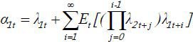
one. Figures 2 and 3 present the estimated α1t (the time-varying coefficient for
) along with the 95% confidence bands under the PPP.9 The estimated cointegration parameters are far from constant and are always above
one. Figures 2 and 3 present the estimated α1t (the time-varying coefficient for  ) and α2t (the time-varying coefficient for
  ) under the monetary model. Again, the estimated cointegration coefficients are not
constant at all, but they have signs consistent with the standard monetary model in
most cases.
) under the monetary model. Again, the estimated cointegration coefficients are not
constant at all, but they have signs consistent with the standard monetary model in
most cases.
 UNDER THE PPP
 UNDER THE MONETARY MODEL
 UNDER THE MONETARY MODEL
Figure 4 compares the cointegration errors under the PPP with the [1, −1] cointegration vector and errors under the PPP with time-varying cointegration coefficients. Similarly, Figure 5 compares the cointegration errors under the monetary model between the [1, −1, 1] cointegration vector and time-varying cointegration coefficients. Both figures show that the residuals from the time-varying cointegration regressions appear to be much more stable and stationary than those from the restricted cointegration vectors. This finding is consistent with the results in Table 4.
VI. The Predictability of the Exchange Rate and the Time-varying Cointegration Approach
The results of various specification tests indicate that data in Korea are favorable to time-varying cointegration approach. Because the time-varying cointegration approach enables both the PPP and the monetary model to pass those specification tests, we compare the predictive abilities of these models to forecast the exchange rate in this section. That is, we check whether deviations from the time-varying long-run equilibrium value of the exchange rate under the PPP or the monetary model are useful in predicting future changes of the exchange rate.
A. In-sample Analysis
In order to determine the predictive abilities of the models, we consider the following univariate predictive regression:

where 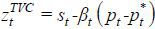 under the PPP, and
 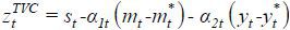 under the monetary model. As the exchange rate moves toward long-run equilibrium
over time, γκ should be negative.
under the monetary model. As the exchange rate moves toward long-run equilibrium
over time, γκ should be negative.
The results of the in-sample analysis are presented in Table 5. γk (the slope coefficient in the predictive regression) always has correct signs and is significant regardless of forecast horizons or regardless of the underlying model used. The PPP model has impressive predictive power for horizons shorter than one year. Specifically, the PPP model can explain 31% of the variation in the exchange rate at a six-month horizon. As horizons become longer, however, the monetary model shows better forecasting ability. We also run the following regression to determine whether the combination of the PPP and the monetary model improves the predictive power:
TABLE 5
PREDICTIVE REGRESSIONS: IN-SAMPLE ANALYSIS
Note: Numbers in parentheses are t-statistics based on Newey-West standard errors.

where 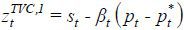 and
and 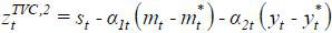 . As shown in the last three-columns of Table 5, γ1,k is significant over shorter horizons, while γ2,k is significant over longer horizons. However, the combination of the two models does
not improve the predictive ability much over the PPP for short horizons and/or over
the monetary model for long horizons. This implies that the time-varying PPP relationship
is the dominant reason for the time-varying monetary model among four structural equations
(Equations (4) – (7)) under the monetary model.
. As shown in the last three-columns of Table 5, γ1,k is significant over shorter horizons, while γ2,k is significant over longer horizons. However, the combination of the two models does
not improve the predictive ability much over the PPP for short horizons and/or over
the monetary model for long horizons. This implies that the time-varying PPP relationship
is the dominant reason for the time-varying monetary model among four structural equations
(Equations (4) – (7)) under the monetary model.
B. Out-of-sample Analysis
We also compare the out-of-sample performance of both models to that of the random walk without drift, which has been the benchmark for assessing the out-of-sample performance of exchange rate models in many studies since Meese and Rogoff (1983). In the out-of-sample analysis, time-varying cointegration errors are constructed using data up to January of 2005, and then the predictive regression in Equation (13) is run to estimate γ0,k and γk. Using the estimated values of γ0,k and γk and the last observation of cointegration errors, forecasts are made for future changes in the exchange rate. We repeat these steps while keeping the window size constant. When comparing the out-of-sample performance of the time-varying PPP or the time-varying monetary model to that of a random walk model, we employ the Clark and West (2007) test statistic. The null hypothesis is that two competing forecasting models have an equal mean-squared prediction error. We construct the Clark-West test statistic so that it has a significantly positive sign if the regression model with time-varying cointegration errors exhibits superior predictive power in relation to the random walk model.
Table 6 reports the test results. Unlike the impressive results in the in-sample analysis, the time-varying PPP and the time-varying monetary model outperform the random walk model at the 10% level only when the forecast horizon reaches 48 months. Even if the time-varying PPP and the time-varying monetary model are combined, the out-of-sample performance does not improve at all. This deterioration of the performance of both time-varying models in the out-of-sample analysis, however, may not result from the nature of those models. Instead, it may be related to the loss of power resulting from the smaller sample size for the estimation in the out-of-sample analysis, as emphasized by Inoue and Kilian (2004) and Bacchetta et al. (2010). This issue should be further investigated with more observations in the future.
TABLE 6
PREDICTIVE REGRESSIONS: OUT-OF-SAMPLE ANALYSIS: COMPARISON WITH RANDOM WALK
Note: Numbers in parentheses are p-values.
We also compare the out-of-sample performances of time-varying models with those of the counterparts based on constant cointegration models. The results are reported in Table 7. Consistent with Table 6, the Clark-West test statistic is designed to have a significantly positive sign if the regression model with time-varying cointegration errors exhibits superior predictive power to the corresponding constant cointegration model. The constant cointegration approach shows significantly better out-of-sample performances in short horizons than the time-varying cointegration approach, regardless of underlying macroeconomic models. As the forecast horizon increases, however, the time-varying models show better out-of-sample forecast ability regardless of underlying macroeconomic models. The superiority of the predictability from the time-varying model over the counterparts from the constant cointegration model becomes significant at horizons longer than one or two years.
TABLE 7
PREDICTIVE REGRESSIONS: OUT-OF-SAMPLE ANALYSIS: COMPARISON BETWEEN TIME-VARYING COINTEGRATION MODEL AND CONSTANT COINTEGRATION MODEL
Note: Numbers in parentheses are p-values.
Finally, we compare the out-of-sample performances among the time-varying PPP, the time-varying monetary model, and the combination of the two. The first two columns of Table 8 show horse race results between the time-varying PPP and the time-varying monetary model. The time-varying PPP outperforms the time-varying monetary model at all horizons except for the six-month horizon, and the gap in the forecast performance is significant at 12–36 month horizons according to the Diebold-Mariano test. Similarly, the time-varying PPP always shows better out-of-sample performance against the combination of the two models except with a six-month horizon, as shown in the last two columns of Table 8. Again, the superior performance of the time-varying PPP relative to the combined model is significant at 12–36 month horizons according to the Diebold-Mariano test. Although the time-varying PPP shows the best out-of-sample performance, the results should be interpreted with caution, as argued by Inoue and Kilian (2004) and Bacchetta et al. (2010).
VII. Discussion
This paper shows that when cointegration coefficients are allowed to vary over time, both the PPP and the monetary model can pass various specification tests, implying that macroeconomic variables based on those models are tightly linked with the exchange rate in Korea. When the abilities to predict future exchange rates between those models based on time-varying cointegration coefficients are compared, the in-sample analysis shows that the time-varying PPP (monetary model) shows better predictive power with horizons shorter (longer) than one year. The results of the out-of-sample analysis indicate that the time-varying PPP performs better when used to predict future changes in the exchange rate.
In addition to these findings, the movements of time-varying coefficients appear to have some signaling power for the Korean economy. The time-varying cointegration coefficient based on the PPP increased around the periods of the Asian currency crisis and the global financial crisis, which may reflect the drastic depreciation of the Korean currency around the time of those crises. The seemingly upward-sloping trend in the time-varying coefficients based on the PPP in Figure 1 suggests a depreciation of the real exchange rate resulting from the slowdown of the growth in the Korean economy.10 The time-varying coefficients based on the monetary model in Figures 2 and 3 also behaved abnormally around these two crises. The coefficients of the relative money (for the relative income) are usually positive (negative) as the theoretical model predicts, but they became negative (positive) around the two crises, implying a drastic depreciation of the Korean currency as compared with fundamentals at those times.
Notes
Studies such as Stock and Watson (1993) and Mulligan and Sala-i-Martin (2000) show that the money demand function has unstable coefficients. Clarida et al. (2000) and Kim and Nelson (2006) demonstrate that monetary policy rules have also shifted over time.
As an exception, Kim and Jei (2013) and Kim et al. (2009) examine time-varying cointegration relationships among variables under the PPP hypothesis for Asian countries.
These unobserved processes are assumed to follow nonstationary processes in Engel and West (2005), as they were not able to find evidence of cointegration between the exchange rate and observable fundamentals. Using the time-varying cointegration approach, however, we find cointegration evidence of these variables, as shown in the next section. As a result, we assume stationarity with regard to these unobserved components.
Due to data availability, the index for mining and manufacturing industrial products is used for the Korean real income data.
Although some studies advocate the use of the Producer Price Index (PPI) to examine the PPP hypothesis, our results are not sensitive regarding whether CPI or PPI data are used in the analyses. Results based on the PPI are available upon request.
The web address for the Bank of Korea is http://ecos.bok.or.kr/. The web address for the Federal Reserve Bank of St. Louis is https://www.stlouisfed.org/.
Following Stock and Watson (1993), we employ dynamic least squares to have optimal estimates of cointegration parameters. The estimated results for first-difference terms are not reported to conserve space, but are available upon request.
The Bierens and Martins test statistics and p-values in parentheses shown in Table 4 are those with three lag orders and two Chebyshev polynomials.
References
(1991). Heteroskedasticity and Autocorrelation Consistent Covariance Matrix Estimation. Econometrica, 59, 817-858, https://doi.org/10.2307/2938229.
, & (2013). On the Unstable Relationship between Exchange Rates and Macroeconomic Fundamentals. Journal of International Economics, 91, 18-26, https://doi.org/10.1016/j.jinteco.2013.06.001.
, & (2001). Long Horizon Exchange Rate Predictability? Review of Economics and Statistics, 83, 81-91, https://doi.org/10.1162/003465301750160054.
, & (2010). Time-Varying Cointegration. Econometric Theory, 26, 1453-1490, https://doi.org/10.1017/S0266466609990648.
, & (2001). Currency Traders and Exchange Rate Dynamics: A Survey of the US Market. Journal of International Money and Finance, 20, 439-471, https://doi.org/10.1016/S0261-5606(01)00002-X.
, & (1995). Banking on Currency Forecasts: How Predictable is Change in Money? Journal of International Economics, 38, 161-178, https://doi.org/10.1016/0022-1996(94)01334-O.
, , & (2000). Monetary Policy Rules and Macroeconomic Stability: Evidence and Some Theory. Quarterly Journal of Economics, 115, 147-180, https://doi.org/10.1162/003355300554692.
, & (2007). Approximately Normal Tests for Equal Predictive Accuracy in Nested Models. Journal of Econometrics, 138, 291-311, https://doi.org/10.1016/j.jeconom.2006.05.023.
, & (2005). Exchange Rates and Fundamentals. Journal of Political Economy, 113, 485-517, https://doi.org/10.1086/429137.
, & (1987). Co-Integration and Error Correction: Representation, Estimation and Testing. Econometrica, 55, 251-276, https://doi.org/10.2307/1913236.
. (1988). Statistical Analysis of Cointegrating Vectors. Journal of Economic Dynamics and Control, 12, 231-254, https://doi.org/10.1016/0165-1889(88)90041-3.
. (1999). Exchange Rates and Monetary Fundamentals: What Do We Learn from Long-Horizon Regressions? Journal of Applied Econometrics, 14, 491-510, https://doi.org/10.1002/(SICI)1099-1255(199909/10)14:5<491::AID-JAE527>3.0.CO;2-D.
, , & (2009). The Purchasing Power Parity of Southeast Asian Currencies: A Time-varying Coefficient Approach. Economic Modelling, 26, 96-106, https://doi.org/10.1016/j.econmod.2008.05.009.
, & (2013). Empirical Test for Purchasing Power Parity Using a Time-varying Parameter Model: Japan and Korea cases. Applied Economics Letters, 20, 525-529, https://doi.org/10.1080/13504851.2012.689109.
, & (2006). Estimation of a Forward-Looking Monetary Policy Rule: A Time-Varying Parameter Model using Ex-Post Data. Journal of Monetary Economics, 53, 1949-1966, https://doi.org/10.1016/j.jmoneco.2005.10.017.
, , , & (1992). Testing the Null Hypothesis of Stationarity Against the Alternative of a Unit Root: How Sure are We that Economic Time Series Have a Unit Root? Journal of Econometrics, 54, 159-178, https://doi.org/10.1016/0304-4076(92)90104-Y.
(1996). Numerical Distribution Functions for Unit Root and Cointegration Tests. Journal of Applied Econometrics, 11, 601-618, https://doi.org/10.1002/(SICI)1099-1255(199611)11:6<601::AID-JAE417>3.0.CO;2-T.
, , & (1999). Numerical Distribution Functions of Likelihood Ratio Tests for Cointegration. Journal of Applied Econometrics, 14, 563-577, https://doi.org/10.1002/(SICI)1099-1255(199909/10)14:5<563::AID-JAE530>3.0.CO;2-R.
, & (1983). Empirical Exchange Rate Models of the Seventies: Do They Fit Out of Sample? Journal of International Economics, 14, 3-24, https://doi.org/10.1016/0022-1996(83)90017-X.
, & (2000). Extensive Margins and the Demand for Money at Low Interest Rates. Journal of Political Economy, 108, 961-991, https://doi.org/10.1086/317676.
, & (2013). Exchange Rate Predictability and a Monetary Model with Time-varying Cointegration Coefficients. Journal of International Money and Finance, 37, 394-410, https://doi.org/10.1016/j.jimonfin.2013.05.003.
(1992). Canonical Cointegration Regressions. Econometrica, 60, 119-143, https://doi.org/10.2307/2951679.
, & (1990). Asymptotic Properties of Residual Based Tests for Cointegration. Econometrica, 58, 165-193, https://doi.org/10.2307/2938339.
(1994). A Residual-based Test of the Null of Cointegration Against the Aalternative of No Cointegration. Econometric Theory, 10, 91-115, https://doi.org/10.1017/S0266466600008240.
, & (1993). A Simple Estimator of Cointegrating Vectors in Higher Order Integrated Systems. Econometrica, 61, 783-820, https://doi.org/10.2307/2951763.