- P-ISSN 1738-656X
- E-ISSN 2586-4130

This paper compares the monetary policy problem in open economies with that in closed economies. It is found that the monetary policy problems in open and closed economies are isomorphic even in the presence of distortions in a steady state and hence the optimal monetary policies have similar properties. On the other hand, the monetary policy maker in open economies has a distorted incentive to manipulate the terms-of-trade. Because of the additional distortion in open economies, there exist gains from international monetary policy cooperation even in the case of a unit intertemporal elasticity of substitution, in contrast to the literature that abstracts from distortions in a steady state. Also, it is found that in the presence of distortions inflation bias is decreasing in openness, which is line with empirical evidence. In addition, this paper presents a simple transformation so that methods in closed-economy models are easily applicable to open-economy models.
Monetary Policy, Isomorphism, Distortion, Inflation Bias, International Cooperation, 통화정책, 같은꼴 사상, 왜곡, 인플레이션 편의, 국제협력
E52, E61, F42
This paper compares the monetary policy problem in open economies with that in closed economies. It has been questioned whether the inward-looking monetary policy that lets the exchange rate move freely is better than the fixed-exchange-rate monetary policy. The literature claimed that the former is better than the latter by showing that the monetary policy problem in open economies is isomorphic to that in closed economies when there is no distortion in a steady state. On the other hand, in open economies there exist additional distortions related to terms-of-trade manipulation and thus the monetary policy maker faces a different problem. To explore the similarities and differences between open- and closed-economy monetary policies, one needs to compare the monetary policy problems in the presence of distortions. It is the main objective of this paper.
The contribution of this paper is three-fold. First, this paper formally shows that monetary policy problems in open and closed economies are isomorphic in richer environments. Clarida, Galí, and Gertler (2001, 2002) and Galí and Monacelli (2005) reported the isomorphism when there is no distortion in a steady state in that flexible-price equilibrium is efficient without disturbances. The main implication of the papers is that an inward-looking monetary policy is optimal. In other words, the monetary policy maker should be concerned only about domestic inflation and output gap, and then the exchange rate will be adjusted so that international resource allocations are efficient. Although some coefficients of equilibrium conditions are different, there is a tradeoff between domestic inflation and output gap stabilization as in closed economy models. That is, the monetary policy problems in open and closed economies are structurally, and thus essentially, the same. This paper extends their results such that the monetary policy problems in open and closed economies are isomorphic even in the presence of distortions in a steady state. This extension is important because distortions that the monetary policy maker faces in open and closed economies may be different as reported in Corsetti and Pesenti (2001, 2005) and Benigno and Benigno (2003). In contrast to Clarida, Galí, and Gertler (2002) and Benigno and Benigno (2003), this paper allows home bias in consumption and thus the real exchange rate is not trivially determined. Home bias is essential in a small open economy model since, otherwise, domestic production of a small open economy does not have any influence on welfare.
The main reason why the literature on the isomorphism had focused on environments without distortions in a steady state is that in those environments the standard linear-quadratic approximation method is easily applicable. In contrast, this paper presents a transformation in the level of monetary policy problems and does not rely on the linear-quadratic approximation. Thus, we can compare the monetary policy problems in open and closed economies directly, whereas the earlier literature has compared the solutions to monetary policy problems. The thing is that to show the isomorphism, one does not need to obtain and compare the final solutions to monetary policy problems.
Second, this paper explicitly shows that the monetary policy maker tries to reduce output because of additional distortion in open economies. Corsetti and Pesenti (2001, 2005) also reported the incentive for monetary contraction in open economies. Since the monetary policy maker can affect overall price level of domestic product, he has an incentive to manipulate the terms-of-trade such that by revaluating the domestic currency, domestic product becomes expensive and hence labor supply of domestic households may be reduced. The papers showed this idea by examining how monetary policy surprise affects allocations. Rational individuals, however, understand the incentive of the monetary policy maker and thus will respond for that. Corsetti and Pesenti (2001, 2005) modeled nominal rigidity as prices are set one period in advance. In their setting, indeed, no rational expectation equilibrium exists when the monetary policy maker tries to manipulate the terms-of-trade discretionally as reported by Benigno and Benigno (2003). In contrast, this paper models nominal rigidity by a Calvo-pricing technology and obtains the incentive in rational-expectation equilibrium. Benigno and Benigno (2003) identified the conditions under which price stabilization is an optimal monetary policy. That is, the paper essentially studied what fiscal instrument eliminates monetary policy distortions. In contrast, this paper explores the monetary policy maker’s incentive for a given fiscal policy, which may not be optimal, and thus shows how distortions affect the monetary policy problem in open economies. De Paoli (2009) studied the optimal monetary policy in a small open economy when distortions from monopolistic competition and terms-of-trade manipulation are both present. The paper relies on numerical analysis to see the effects of terms-of-trade manipulation in addition to those of monopolistic competition. In contrast, this paper analytically shows how the two incentives are combined.
Third, this paper presents a simple transformation so that methods in closed economy models are easily applicable to open economy models. Given the extensive literature on monetary policy in closed economy models (for example, Clarida, Galí, and Gertler [1999] and Woodford [2003] among others), one may apply the transformation to those models to get results in open economy models directly (see Corsetti, Dedola, and Leduc [2011] for a recent survey on monetary policy in open economies). Although the model in this paper is highly stylized, it can be a good benchmark to understand basic intuitions. With relaxed assumption in open economy models, numerical approach may be required. In those situations, the results in this paper can be a good starting point, for example, in the homotopy continuation method.
This paper is organized as follows. Section II presents the model and Section III derives equilibrium conditions. Section IV presents the isomorphism between monetary policy problems in open and closed economies in each case of cooperative and non-cooperative monetary policy. Section V illustrates the results with applications and Section VI concludes.
There are two countries, Home and Foreign, whose measures are, respectively, γ and 1−γ . If γ is small-enough, then Home is a small open economy. Products are differentiated and indexed by f . Good f in [0,γ] is produced at Home while good f in (γ,1] is at Foreign.
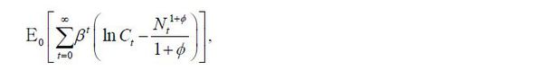
Households’ preference depends on their consumption and labor supply. As is standard in New Keynesian models, we assume that consumption and labor supply are separable in the utility function. We assume further that the intertemporal elasticity of substitution of consumption is one. This value is within a standard range and commonly used in the real-business cycle and New Keynesian literature. When the utility function is separable, a unit intertemporal elasticity of substitution is a condition consistent with a balanced growth path. Therefore, the preference is represented by
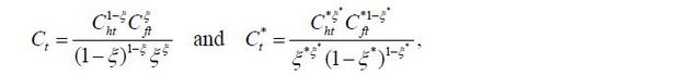
where Et denotes the expectation operator given information up to period t and β the discount factor. Ct is consumption and Nt labor supply in period t. Ct is an aggregate of Home product Cht and Foreign product Cft . The elasticity of substitution between Home and Foreign products is also assumed to be one. Due to this assumption, the monetary policy problem becomes more tractable and can be solved analytically. Indeed, Galí and Monacelli (2005) and Faia and Monacelli (2008) reported that the monetary policy that stabilizes domestic price is optimal in a small open economy under the elasticity assumption. Home and Foreign consumption aggregates are, respectively,
where ξ = (1−γ)η and ξ* = γη for η ∈ [0,1] . η measures openness of the economies. When η is equal to zero, the two countries are closed economies and households consume domestic products only. In contrast, when η is equal to one, they are fully open and the consumption weights are the same with the countries’ sizes. When η is less than one, households are biased toward domestic products. In the limit case that γ goes to zero with positive η , Home is a small open economy and Foreign is a closed economy. In the literature, two country models sometimes abstract from home bias in consumption. Home bias is, however, essential in a small open economy model because, without the assumption, Home product is negligible in consumption baskets and thus both Home and Foreign agents do not care about the amount of Home production.
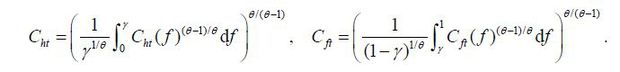
The elasticity of substitution among Home products and that among Foreign products are both θ > 1. That is, the aggregators of Home and Foreign products are, respectively,
Households’ budget constraint in state ht is
where Bt+1(ht+1) is the purchase of the bond that pays one unit of domestic currency in state ht+1 and Mt(ht+1) is the bond price. Households receive firms’ profits and government transfers.
Household h is a monopolistic competitive supplier of type-h labor and sets a wage rate Wt(h) in each period t. Labor input is aggregated as  for wage markup
  ≥ 1 , which is assumed to be exogenous. We assume flexible wage so that it can be
reset in each period. Every household faces the same problem of wage-setting, and
the household optimization implies that the real wage in equilibrium is
≥ 1 , which is assumed to be exogenous. We assume flexible wage so that it can be
reset in each period. Every household faces the same problem of wage-setting, and
the household optimization implies that the real wage in equilibrium is  . That is, the wage is equal to the marginal value of labor supply, which is equal
to the marginal rate of substitution between consumption and labor supply, multiplied
by the wage markup. Fluctuation of plays a role in New Keynesian models as a cost-push shock, which implies a short-run trade-off between output and inflation stabilization.
Similarly,
. That is, the wage is equal to the marginal value of labor supply, which is equal
to the marginal rate of substitution between consumption and labor supply, multiplied
by the wage markup. Fluctuation of plays a role in New Keynesian models as a cost-push shock, which implies a short-run trade-off between output and inflation stabilization.
Similarly,  is Foreign wage markup.
Home firm f ∈ [0,γ] produces with a constant-returns-to-scale technology Yt(f) = AtNt(f) , where At is a country-specific productivity. Similarly,  denotes Foreign firms’ productivity. Firms receive a subsidy τ for each employment (they pay a tax if τ < 0 .). Thus, firms’ nominal cost for unit employment is (1−τ)Wt . In the terms of modeling, it doesn’t matter whether firms or workers receive subsidy.
Moreover, sales subsidy to firms or consumption subsidy to households for domestic
products also yields the same conclusion.
denotes Foreign firms’ productivity. Firms receive a subsidy τ for each employment (they pay a tax if τ < 0 .). Thus, firms’ nominal cost for unit employment is (1−τ)Wt . In the terms of modeling, it doesn’t matter whether firms or workers receive subsidy.
Moreover, sales subsidy to firms or consumption subsidy to households for domestic
products also yields the same conclusion.
Nominal rigidity is modeled by the assumption of a standard Calvo pricing technology
that each firm cannot reset its price with probability α as introduced by Calvo (1983). The event is independent across firms and over time. We assume that a firm sets
a single price in its own currency for both Home and Foreign markets. This implies
that the law of one price holds for every individual product at all time,  and
and  , where the nominal exchange rate St is the Home currency price of Foreign currency.
We assume that financial market is complete. We will, however, show that the financial market completeness is irrelevant with a certain initial condition.
We assume that disturbances (At,  ) t t A m and (, ) t t A m follow Markov processes. This assumption is not critical but necessary to
write the monetary policy problem in a recursive form.
) t t A m and (, ) t t A m follow Markov processes. This assumption is not critical but necessary to
write the monetary policy problem in a recursive form.
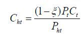
When the elasticity of substitution between Home and Foreign products is one, households’ optimization implies that they spend a constant share of their total expenditure for each product. Home and Foreign demands for Home and Foreign products are, respectively,
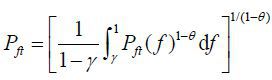
where Home and Foreign consumer price indices are, respectively, Pt =  and
and  . Demand functions for individual firm’s product are
where Home consumer price indices for Home and Foreign products are, respectively,
By the assumption that the law of one price holds, Foreign counterparts are  = StPht and
  = St .
We have assumed that financial market is complete. We will, however, show that the
assumption is not crucial. We start with the complete financial market. A risk sharing
condition is that the real exchange rate is proportional to the ratio of marginal
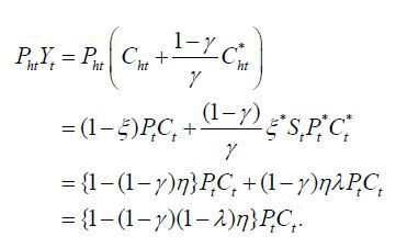
utilities of consumption,  = λPtCt for some λ . The constant λ depends on initial conditions. Then the value of Home output in period t is
That is, the value of output is always proportional to that of consumption. In particular, if λ =1 , they are always the same. In that case, both trade and investment income account balances are always zero and so is current account balance. Thus, equilibrium under the complete financial market is the same with that under financial autarky. In other words, the assumption about financial market is irrelevant to the equilibrium allocation. To relax financial market completeness, the literature on open economy models often assumes that only non-contingent bonds are tradable. If countries have no initial debts, they would not have any debt in the future, either. That is, model’s implications are the same in all the three financial market structures (complete financial market, financial autarky, and bond-only market) with a certain initial condition. We prefer the initial condition in that, on the one hand, it is usually assumed and, on the other hand, results do not depend on the model’s specification on financial market structure.
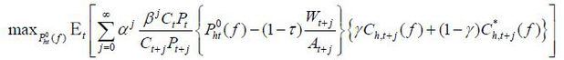
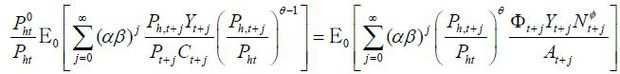
Now we move on to firms’ price-setting problem. The problem of a firm that has an opportunity to reset its price in period t is
subject to the sequence of demand functions. The additional discount factor αj reflects the probability that the firm’s price set in period t cannot be reset until period t+j. One can see that all firms setting new prices face the same problem. Thus, we drop
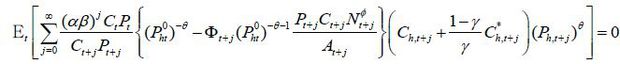
the index f in the optimal reset price. Note, also, that the law of one price implies that Pht(f) / Pht = (f) / for all f in [0,γ]. Then, the first order condition is
where Φt ≡ (1 − τ)μp . Φt represents distortions of the economy, that is, distortionary subsidy, price markup,
and wage markup. By the market clearing condition, γYt = γCht + (1 − γ) for all t, we have
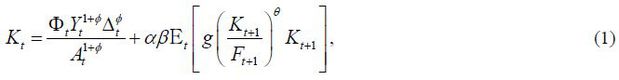
Since the values of output and consumption are always the same, Ph,t+jYt+j = Pt+jCt+j , we obtain the optimality condition
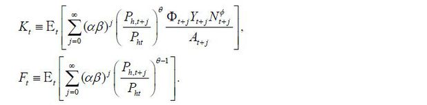
where we define
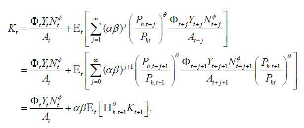
That is, the price is a weighted average of current and future marginal costs multiplied by markups. In these equations, we can see that the marginal cost does not depend on Foreign variables. As explained in Clarida, Galí, and Gertler (2002), a rise in Foreign output affects the marginal cost in two channels, terms-of-trade and wealth effects. With a unit elasticity of substitution, the two effects are exactly offset. We may rewrite these equations recursively as
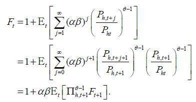
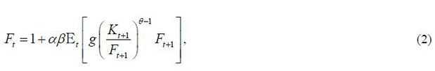
and
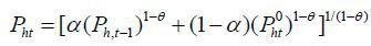
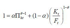
Since the aggregate price of Home products evolves as
dividing both sides by Pht we have
where Πht is the gross inflation rate of Home product in period t. Rewriting the equation, we obtain  , where
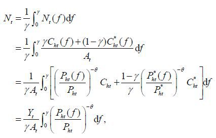
The labor market clearing condition is
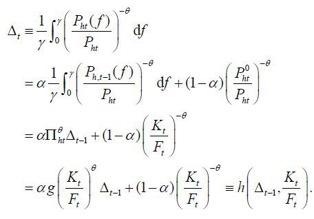
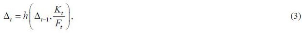
where the last equality follows from Pht(f) / Pht = (f) / and γYt = γCht + (1 − γ) . That is, the aggregate labor supply is Nt = YtΔt / At , where Δt denotes price dispersion defined as
The more price dispersion, the more labor supply required given output and productivity. Price dispersion, hence, represents the inefficiency due to nominal rigidity.
In sum, equilibrium conditions include
There are five variables in the four equations above. The remaining equation is the monetary policy function. As is standard in the optimal policy literature, we do not explicitly express the policy function. We, instead, describe the relationship among the endogenous variables in equilibrium.
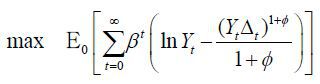
For a normative analysis of the monetary policy, we set the objective function of
the policy maker explicitly based on individuals’ preference. That is, a benevolent
policy maker is to maximize the expected utility of households subject to private
agents’ optimality conditions. The welfare function of Home policy maker is, therefore,
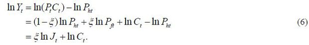
It is convenient to rewrite the welfare function in terms of output instead of consumption. The real exchange rate Qt (the price of Foreign consumption basket in terms of Home consumption basket) and terms-of-trade Jt (the price ratio of imported goods to exported goods) have the following relationship.
Then we can rewrite the risk sharing condition  as
as
Since the values of Home output and consumption are always the same,
Its Foreign counterpart is
Solving equations (5), (6), and (7) simultaneously, we obtain
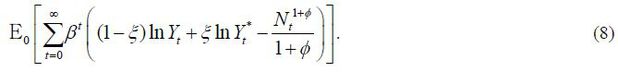
Therefore, the objective function of Home policy maker is
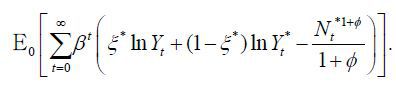
Its Foreign counterpart is
Now, we are ready to compare monetary policies in open and closed economies.
If ξ = 0 , then Home is a closed economy. The consumer price and domestic price are identical and so are inflations, Πht = Πt . Therefore, the monetary policy problem is
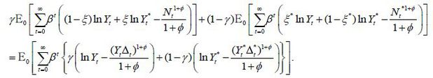
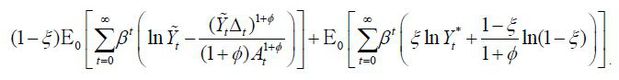
The monetary policy makers in the two countries maximize the weighted sum of the expected utilities of the two countries. We assume that every individual is equally weighted. That is, the weights of the two countries are proportional to the countries’ sizes, γ and 1 − γ . Then the objective function is
where we used γ(1 − ξ) + (1 − γ)ξ* = γ and γξ + (1 − γ)(1 − ξ*) = 1 − γ . Note that Home and Foreign variables in the objective function are additively separable. Also, the set of equilibrium conditions are divided into equations with Home variables and with Foreign variables. Thus, the optimal cooperative monetary policy should solve
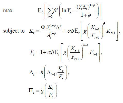
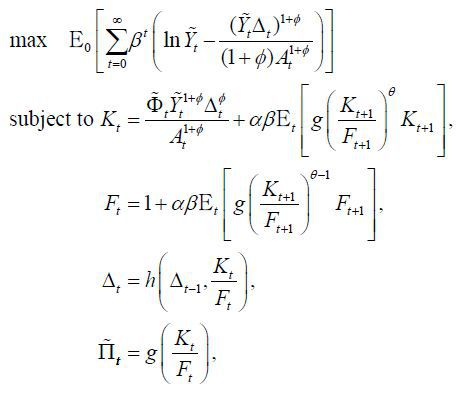
subject to (1), (2), (3), and (4). The only difference from the monetary policy problem in closed economies is domestic inflation rather than CPI inflation.
Proposition 1 (Cooperative monetary policy) The monetary policy problem in open economies is isomorphic to that in closed economies with a transformation Πt → Πht .
Remark The key reason for the isomorphism is that Home marginal cost does not depend on Foreign variables explicitly in open economies. Firms’ price setting is summarized by Kt and Ft, from which we can see the optimal reset price is the weighted average of current and future marginal costs. In general, Foreign production may affects Home marginal cost through two channels. First, if Foreign output increases, Home output becomes relatively scarce and hence the terms-of-trade improves. Given Home consumption level, it reduces Home marginal cost. Second, if Foreign output increases, so does Home consumption. Then the marginal value of leisure increases and thus labor input becomes more expensive. Therefore, the wealth effect by a rise in Foreign output implies higher Home marginal cost. As reported in Clarida, Galí, and Gertler (2002), the two effects are exactly offset when the elasticity of substitution is one. Thus, Home marginal cost does not depend on Foreign output directly. The property holds regardless of distortions, which is the main factor for Proposition 1.
The result in Clarida, Galí, and Gertler (2002) can be directly implied by Proposition 1. Compared with Proposition 1, the paper assumed no distortions in a steady state and showed their results in an approximated problem. We could extend their results because we compared not the solutions to the policy problems but the policy problems themselves.
The monetary policy maker maximizes Home households’ expected utility given Foreign agents’ decision. Now we will show a transformation that links the monetary policy problem in open economies to that in closed economies. Let Ỹt ≡ (1 − ξ)−1/(1+ϕ)Yt . Then we may rewrite the objective function as
Note that the second term is independent of Home monetary policy. Thus, the problem of the non-cooperative policy maker can be rewritten as
where  and
and  . The transformed problem has the same structure with that of the monetary policy
problem in closed economies.
. The transformed problem has the same structure with that of the monetary policy
problem in closed economies.
Proposition 2 (Non-cooperative monetary policy) The monetary policy problem in open economies is isomorphic to that in closed economies with a transformation (Yt, Φt, Πt) → ((1 − ξ)-1/(1+ϕ)Yt, (1 − ξ)Φt, Πht) .
Compared to the problem in closed economies, there is an additional term in distortions (1 − ξ) . That is, the monetary policy maker in open economies behaves as if there is a distortionary employment subsidy ξ . In other words, Home output is produced too much due to the subsidy in the view point of the policy maker and thus should be reduced at optimum.
The welfare function, equation (8), shows that only (1 − ξ) portion of domestic output is consumed by Home households in equilibrium. Thus, the tradeoff between consumption and labor supply is different in open economies. In particular, labor supply in open economies should be less than that in closed economies. That is, the open-economy monetary policy should be more contractionary.
To illustrate the results in this paper, we present three applications. The first application shows that the results in the early literature can be easily driven by the transformation in this paper. The second application explores differences between the monetary policy in open and closed economies. The main difference is the distortions that the monetary policy maker faces. Due to this difference, there are gains from monetary policy cooperation, which is a different implication from Clarida, Galí, and Gertler (2002). The final application shows how to obtain inflation bias in open economies with results in closed economy models.
First, in the cases of the monetary policy cooperation, Proposition 1 says that the only difference in monetary policies is inflations that the policy maker targets. Thus, without distortions in a steady state, the result that the monetary policy maker in closed economies balances inflation and output gap stabilization continues to hold in open economies in that the policy maker balances domestic inflation and output gap stabilization.
Now we move on to the cases of the non-cooperative monetary policy. Suppose that fiscal
policy is set such that there is no distortion in a steady state,  = 1 or (1 − ξ)(1 − τ)μpμw = 1. Note that the log deviations from the efficient output do not change by the
transformation, ln Ỹt − ln Ỹe = ln Yt − ln Ye , where Ye is output in the flexible price equilibrium. Therefore, if one expresses the monetary
policy in terms of output gap and inflation, the solutions to the monetary policy
problems in open and closed economies would be the same except that in open economies
domestic inflation is used instead of consumer price inflation. Again, in equilibrium
the monetary policy would balance domestic inflation and output gap stabilization.
Galí and Monacelli (2005) assumed that the wage markup is always one in a small open economy. Remind that as
γ goes to zero, Home is a small open economy and ξ = (1 − γ)η → η . The paper further assumed that (1 − η)(1 − τ)μp = 1. Then
= 1 or (1 − ξ)(1 − τ)μpμw = 1. Note that the log deviations from the efficient output do not change by the
transformation, ln Ỹt − ln Ỹe = ln Yt − ln Ye , where Ye is output in the flexible price equilibrium. Therefore, if one expresses the monetary
policy in terms of output gap and inflation, the solutions to the monetary policy
problems in open and closed economies would be the same except that in open economies
domestic inflation is used instead of consumer price inflation. Again, in equilibrium
the monetary policy would balance domestic inflation and output gap stabilization.
Galí and Monacelli (2005) assumed that the wage markup is always one in a small open economy. Remind that as
γ goes to zero, Home is a small open economy and ξ = (1 − γ)η → η . The paper further assumed that (1 − η)(1 − τ)μp = 1. Then  for all t. In closed economies without a cost-push shock, price stabilization is an optimal
monetary policy. According to the transformation in this paper, the open-economy counterpart
is that domestic price stabilization is an optimal monetary policy, which is the same
with the result in Galí and Monacelli (2005).
for all t. In closed economies without a cost-push shock, price stabilization is an optimal
monetary policy. According to the transformation in this paper, the open-economy counterpart
is that domestic price stabilization is an optimal monetary policy, which is the same
with the result in Galí and Monacelli (2005).
We have shown that in both cases, one can obtain the optimal monetary policy in open economies directly by applying the transformation in this paper. When there is no distortion in a steady state, the optimal monetary policy in open and closed economies are very similar. The subsidy rates for a non-distorted steady state are, however, different in open and closed economies. In the next subsection, we will show that the difference has an important implication.
This paper claims that there exist gains from monetary policy cooperation since the non-cooperative monetary policy maker has an incentive to reduce domestic output. Clarida, Galí, and Gertler (2002) reported that there are no gains from monetary policy cooperation when the intertemporal elasticity of substitution is one. The main point of the paper is that with a unit elasticity of substitution Foreign output level does not affect Home marginal cost. An important assumption of the paper is that fiscal policy eliminates distortions in a steady state in both cooperative and non-cooperative cases. The required subsidy rates are, however, different in the two cases. We, hence, examine whether there exist gains from monetary policy cooperation given fiscal policy.
Proposition 3 Given fiscal policy, there are gains from monetary policy cooperation.
Proof. At optimum the welfare in the cooperative monetary policy cannot be less than that
in the non-cooperative monetary policy. Then it is enough to show that the optimal
non-cooperative monetary policy does not solve the problem of the cooperative monetary
policy. The optimal non-cooperative monetary policy maximizes E0 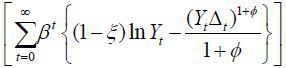 , while the optimal cooperative monetary policy does E0
 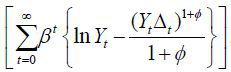 , where the constraints (1), (2), and (3) are common in the two cases. It is obvious
that the solutions to the two problems are different, which completes the proof.
, where the constraints (1), (2), and (3) are common in the two cases. It is obvious
that the solutions to the two problems are different, which completes the proof.
The non-cooperative policy maker induces less output than the cooperative policy maker does. As we have already explained, the reason is that the non-cooperative policy maker ignores Foreign consumption of domestic output. Corsetti and Pesenti (2001, 2005) also reported that the monetary policy maker in open economies has an incentive to manipulate the terms-of-trade. By more contractionary monetary policy, domestic outputs become more expensive and domestic households supply less labor. Although domestic consumption is also reduced, the reduction of labor supply has larger effect on the welfare. Therefore, the monetary policy maker tries to revalue the domestic currency.
The difference from the early literature is that we compare the welfares for given fiscal policy. The main lesson is that in open economies the monetary policy makers have a distorted incentive, which can be eliminated by the international monetary cooperation.
Following from the seminal papers of Kydland and Prescott (1977) and Barro and Gordon (1983), a large literature has studied the problem of inflation bias under discretionary or time-consistent monetary policy. This paper compares inflation bias in open and closed economies. This exercise will illustrate the differences of monetary policies in open and closed economy more clearly. Also, through the exercise one can see how to apply the transformation in this paper.
First, remind that the values of consumption and output are always the same, PtCt = PhtYt . In terms of inflations, we have Πt = ΠhtCt-1Yt / (CtYt-1) . Therefore, the consumer price inflation and domestic inflation are the same in stationary equilibrium, Π = Πh . That is, it is not necessary to distinguish the two inflations in stationary equilibrium.
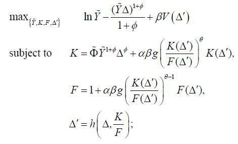
The optimal inflation rate in stationary equilibrium of the Ramsey problem is zero (Π = 1) as shown in Benigno and Woodford (2005). Now consider the optimal inflation rate in stationary equilibrium of the time-consistent policy problem. Since we are focusing on stationary equilibrium, exogenous aggregate variables are assumed to have their steady state values. The equilibrium concept here is a Markov perfect equilibrium. As in Klein, Krusell, and Ríos-Rull (2008), a time-consistent equilibrium consists of a value function V (·) and policy functions {Ỹ(Δ), K(Δ), F(Δ), Δ'(Δ)} such that for all Δ ≥ 1, the policy functions solve
and the value function satisfies
One may think this problem as the monetary policy maker in each period chooses current
monetary policy given the future policy function. That is, the monetary policy maker
cannot commit future policy. Nonetheless, monetary policy in each period affects future
policy through the state variable Δ . The monetary policy maker rationally expects
that the future monetary policy is also optimal given price dispersion in the future
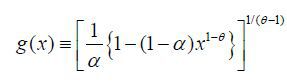
period. The allocations in a stationary equilibrium satisfy Δ = Δ'(Δ) , K = K(Δ) , F = F(Δ) . Then the inflation in the stationary equilibrium is 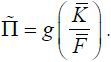 Inflation bias is, therefore,
 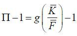 .
.
In a closed economy model, Woodford (2003) showed that when distortion is small (that is,  ), inflation bias is
According to the transformation, inflation bias in open economies is
Proposition 4 Inflation bias is decreasing in openness in the case of small distortions.
Although we conjecture that the proposition holds even in the case of large distortions, we have not proved it yet. Proposition 4 is in line with the empirical result in Romer (1993), which reported that average inflation was lower in more open economies.
Corsetti and Pesenti (2001, 2005) also reported the difference in open and closed economies and less inflationary bias in open economies. The papers, however, examined how unanticipated monetary shocks affect the welfare. The exercise in the papers is useful to understand intuition but inconsistent with rational expectation equilibrium. In their model, agents set price one period in advance. Anticipated inflations do not have any effect on the allocations and thus welfare. That is, if agents understand the policy maker’s incentive and expect contractionary monetary policy, they will change prices accordingly. Indeed, there is no time-consistent rational expectation equilibrium when the monetary policy maker has such an incentive. In contrast, we model nominal rigidity by a Calvo-pricing technology and obtain inflation bias in rational expectation equilibrium.
For calibration we mostly follow Christiano, Eichenbaum, and Evans (2005), which is a key paper in the literature on monetary policy estimation. We let the period length be a quarter and the discount factor β =1.03-0.25 , which implies an annualized real interest rate of 3%. The inverse of the Frisch elasticity of labor supply is set to be one, ϕ = 1. The Calvo-pricing parameter is α = 0.6 , which means that firms change their prices every 2.5 quarters on average. Price and wage markups are μp =1.2 and μw =1.05 .
Christiano, Eichenbaum, and Evans (2005) studied a closed economy and abstracted from fiscal policy. In open economies, we need to calibrate the weight of imports in the consumption basket ξ . The volume of international trade has been growing faster than world production. A reason is the globalization of supply chains as reported in Hummels, Ishii, and Yi (2001). As each country has specialized in particular production stages, trades of intermediate goods have increased rapidly. In such supply chains, a fraction of imports are used not for domestic consumption but for export. For our purpose, we may have to exclude imports for export. In the model in this paper, the values of consumption and output are the same. Hence, ξ is the ratio of imports to GDP, where imports should include only goods and services for domestic use. For calibration we have chosen the Korean economy. The value of imports to Korea is about a half of the value of GDP of Korea. Around 60 percent of imports are for domestic use. Thus, we set ξ = 0.3 .
The remaining parameter is the employment subsidy τ . Note that it does not matter whether firms or workers receive subsidy and that sales subsidy to firms or consumption subsidy to households for domestic products also yields the same conclusion. The thing is the overall distortion by fiscal policy. To calibrate the subsidy, we use the total tax revenue (excluding social security) in the OECD database. The tax revenue of the Korean economy in 2012 is about 20.2% of GDP, which is a little higher than the OECD average. Thus, we set τ = −0.202 .
Then the overall distortion is = 1.06 or 6%, which is far smaller than the corresponding distortion in closed economies,
= 1.51 or 51%. With these parameters the annualized inflation bias in the open economy
is estimated to be about 2.0%, which is far less than that in closed economies, 18.2%.
That is, the monetary policy maker in the open economy has far smaller inflationary
bias. Although the model in this paper is highly stylized and thus the estimates of
inflation bias should be interpreted with caution, this example shows that the distortion
from terms-of-trade manipulation may be as important as the distortions from price
and wage markups.
When distortions are not small-enough, one may not use a perturbation method around an efficient equilibrium. In closed economy models Anderson, Kim, and Yun (2010) obtained inflation bias in a Markov perfect equilibrium using a projection method. The numerical method is also applicable to the problem in open economies by adjusting distortions.
This paper has shown that the monetary policy problem in open economies is isomorphic to that in closed economies even in the presence of distortions. From the transformation, we have learned that the key difference between open and closed economies is the distortion that the monetary policy maker faces. Due to the difference of the distortion, there are gains from monetary policy cooperation, and the time-consistent monetary policy is less inflationary in open economies.
An important assumption in this paper is that the elasticity of substitution is equal to one. Although with other elasticity values one may not obtain the isomorphism analytically and needs to rely on numerical approach, it is important to understand how different distortions are in open and closed economies. Another direction for future work is to relax the assumption of perfect exchange rate pass-through. In the cases of local-currency pricing, Engel (2011) showed that the monetary policy maker should be concerned about currency misalignments and target consumer price inflation instead of domestic inflation. Then it is a key question whether the time-consistent monetary policy is less inflationary in open economies in the cases of imperfect exchange rate pass-through.
, , & . (2010). Using a Projection Method to Analyze Inflation Bias in a Micro-Founded Model. Journal of Economic Dynamics and Control, 34(9), 1572-1581, https://doi.org/10.1016/j.jedc.2010.06.024.
, & (1983). A Positive Theory of Monetary Policy in a Natural Rate Model. Journal of Political Economy, 91(4), 589-610, https://doi.org/10.1086/261167.
, & . (2003). Price Stability in Open Economies. Review of Economic Studies, 70(4), 743-764, https://doi.org/10.1111/1467-937X.00265.
, & . (2005). Inflation Stabilization and Welfare: The Case of a Distorted Steady State. Journal of the European Economic Association, 3(6), 1185-1236, https://doi.org/10.1162/154247605775012914.
(1983). Staggered Prices in a Utility-Maximizing Framework. Journal of Monetary Economics, 12(3), 383-398, https://doi.org/10.1016/0304-3932(83)90060-0.
, , & (2005). Nominal Rigidities and the Dynamic Effects of a Shock to Monetary Policy. Journal of Political Economy, 113(1), 1-45, https://doi.org/10.1086/426038.
, , & . (1999). The Science of Monetary Policy. Journal of Economic Literature, 37(4), 1661-1707, https://doi.org/10.1257/jel.37.4.1661.
, , & . (2001). Optimal Monetary Policy in Open versus Closed Economies: An Integrated Approach. American Economic Review, 91(2), 253-257, https://doi.org/10.1257/aer.91.2.253.
, , & . (2002). A Simple Framework for International Monetary Policy Analysis. Journal of Monetary Economics, 49(5), 879-904, https://doi.org/10.1016/S0304-3932(02)00128-9.
, & . (2001). Welfare and Macroeconomic Interdependence. Quarterly Journal of Economics, 116(2), 421-445, https://doi.org/10.1162/00335530151144069.
, & . (2005). International Dimensions of Optimal Monetary Policy. Journal of Monetary Economics, 52(2), 281-305, https://doi.org/10.1016/j.jmoneco.2004.06.002.
. (2009). Monetary Policy and Welfare in a Small Open Economy. Journal of International Economics, 77(1), 11-22, https://doi.org/10.1016/j.jinteco.2008.09.007.
. (2011). Currency Misalignments and Optimal Monetary Policy: A Reexamination. American Economic Review, 101(6), 2796-2822, https://doi.org/10.1257/aer.101.6.2796.
, & . (2008). Optimal Monetary Policy in a Small Open Economy with Home Bias. Journal of Money, Credit, and Banking, 40(4), 721-750, https://doi.org/10.1111/j.1538-4616.2008.00133.x.
, & . (2005). Monetary Policy and Exchange Rate Volatility in a Small Open Economy. Review of Economic Studies, 72(3), 707-734, https://doi.org/10.1111/j.1467-937X.2005.00349.x.
, , & . (2001). The Nature and Growth of Vertical Specialization in World Trade. Journal of International Economics, 54(1), 75-96, https://doi.org/10.1016/S0022-1996(00)00093-3.
, , & . (2008). Time-Consistent Public Policy. Review of Economic Studies, 75(3), 789-808, https://doi.org/10.1111/j.1467-937X.2008.00491.x.
, & (1977). Rules Rather than Discretion: The Inconsistency of Optimal Plans. Journal of Political Economy, 85(3), 473-492, https://doi.org/10.1086/260580.
. (1993). Openness and Inflation: Theory and Evidence. Quarterly Journal of Economics, 108(4), 869-903, https://doi.org/10.2307/2118453.


 ,
,  ,
,  , and
, and 
 ,
,  for f ∈ [0, γ],
 ,
,  for f ∈ [γ, 1],
 ,
,  .
.
 ,
,
 .
.
 ,
,
 ,
,
 ,
,
 .
.


 .
.